对于想了解Python中的Gauss-Legendre算法的读者,本文将是一篇不可错过的文章,我们将详细介绍pythonlegend,并且为您提供关于CPython3.9python.gram文件-尝
对于想了解Python中的Gauss-Legendre算法的读者,本文将是一篇不可错过的文章,我们将详细介绍python legend,并且为您提供关于CPython 3.9 python.gram文件-尝试使用utf-8文本运行make regen-pegen时出错、openGauss数据库之Python驱动快速入门、PHP中的gmp_legendre()函数、python gaussian,gaussian2的有价值信息。
本文目录一览:- Python中的Gauss-Legendre算法(python legend)
- CPython 3.9 python.gram文件-尝试使用utf-8文本运行make regen-pegen时出错
- openGauss数据库之Python驱动快速入门
- PHP中的gmp_legendre()函数
- python gaussian,gaussian2
")
Python中的Gauss-Legendre算法(python legend)
我需要一些帮助来计算Pi。我正在尝试编写一个将Pi转换为X位数的python程序。我已经从python邮件列表中尝试了几种,但使用起来很慢。我已经阅读了有关Gauss-Legendre算法的文章,并且尝试将其移植到Python中没有成功。
我正在从这里阅读,对于我要去哪里出错,我将不胜感激!
输出:0.163991276262
from __future__ import division import math def square(x):return x*x a = 1 b = 1/math.sqrt(2) t = 1/4 x = 1 for i in range(1000): y = a a = (a+b)/2 b = math.sqrt(b*y) t = t - x * square((y-a)) x = 2* x pi = (square((a+b)))/4*t print pi raw_input()答案1
小编典典您忘记了以下括号
4*t:pi = (a+b)**2 / (4*t)您可以
decimal用来执行更高精确度的计算。
#!/usr/bin/env python from __future__ import with_statement import decimal def pi_gauss_legendre(): D = decimal.Decimal with decimal.localcontext() as ctx: ctx.prec += 2 a, b, t, p = 1, 1/D(2).sqrt(), 1/D(4), 1 pi = None while 1: an = (a + b) / 2 b = (a * b).sqrt() t -= p * (a - an) * (a - an) a, p = an, 2*p piold = pi pi = (a + b) * (a + b) / (4 * t) if pi == piold: # equal within given precision break return +pi decimal.getcontext().prec = 100 print pi_gauss_legendre()输出:
3.141592653589793238462643383279502884197169399375105820974944592307816406286208\ 998628034825342117068
CPython 3.9 python.gram文件-尝试使用utf-8文本运行make regen-pegen时出错
我做过类似您的事情,只是添加了中文关键字。它的工作原理如下:
-
确定错误消息为msg。它位于。\ Tools \ peg_generator \ pegen \ c_generator.py中。打开文件,您可以在AssertionError上方看到re.match行。修改匹配模式以适合您的需求。
-
运行make regen-pegen以重新生成Parser / parser.c。您可能还需要从此文件的第11行开始对reserve_keywords []进行细微更改。以我的情况为例,以“函件”(相当于“ def”)为例,它出现在修改前的第二个{}内部,但是一个中文字符在utf-8中使用3个字节,因此它应该位于第四个{}内部与'def'。还请注意顺序。
祝你好运,玩得开心!

openGauss数据库之Python驱动快速入门
openGauss是一款开源关系型数据库管理系统,采用木兰宽松许可证v2发行。openGauss内核源自PostgreSQL,深度融合华为在数据库领域多年的经验,结合企业级场景需求,持续构建竞争力特性。
可是目前针对于openGauss数据库的Python应用程序的开发少之又少,这其中的一个原因在于不知道用什么驱动来连接该数据库,特别是Python应用程序,在此将给大家介绍如何使用Python驱动连接openGauss数据库,同时翻译了psycopg2的文档:psycopg2中文文档,目前仍在维护和调整中,如果有任何建议,欢迎提PR来进行修正。
一、数据库部署
教程的第一步当然是引导大家部署数据库了,由于openGauss数据库与操作系统有一定的依赖关系,为了屏蔽掉不同操作系统之间部署的区别,我推荐使用Docker来进行部署,部署的脚本如下所示:
# 1.拉取镜像
docker pull enmotech/opengauss

# 2.开启openGauss数据库服务
docker run --name opengauss \
    --privileged=true -d \
    -e GS_USERNAME=gaussdb \
    -e GS_PASSWORD=Secretpassword@123 \
    -p 5432:5432 \
enmotech/opengauss:latest在以上代码中,默认数据库用户名为gaussdb,数据库密码为Secretpassword@123 ,开启服务的端口为5432,相信熟悉Docker的同学一眼就能看明白代码的含义。
可是在此部署的镜像当中只存在一个默认数据库:gaussdb,如果要添加新的数据库节点的话可以使用以下代码:
# 1. 进入运行的Docker容器
docker exec -it opengauss /bin/bash

# 2. 设置环境变量
export GAUSSHOME=/usr/local/opengauss
export PATH=$GAUSSHOME/bin:$GAUSSHOME:$GAUSSHOME/lib:$PATH
export LD_LIBRARY_PATH=$GAUSSHOME/lib:$LD_LIBRARY_PATH
export DATADIR=''/var/lib/opengauss/data''

# 3. 使用gsql登陆openGauss数据库
gsql -U gaussdb -W Secretpassword@123 -d postgres -p 5432

# 4. 创建test_db数据库
CREATE DATABASE test_db WITH ENCODING ''UTF8'' template = template0;

# 5. 重新加载openGauss数据库
gs_ctl reload -D $DATADIR
以上命令执行完毕之后即可创建对应的数据库。
安装教程
要想使用Python驱动在openGauss数据库上开发应用,非常简单,只需要安装以下包即可:
pip install psycopg2-binary安装步骤只需要一步即可,接下来就可以开始应用程序的开发。
Simple Operations with openGauss
为了演示与数据库的基本操作,我将从创建会话连接、创建表、插入数据、修改数据、删除数据以及查询数据等六个方面来演示。
任何数据库的操作都是需要先创建连接来管理对应的事务,openGauss也不例外:
创建会话连接
from psycopg2 import connect


def create_conn():
    """get connection from envrionment variable by the conn factory Returns: [type]: the psycopg2''s connection object """
    env = os.environ
    params = {

        ''database'': env.get(''OG_DATABASE'', ''opengauss''),
        ''user'': env.get(''OG_USER'', ''gaussdb''),
        ''password'': env.get(''OG_PASSWORD'', ''Secretpassword@123''),
        ''host'': env.get(''OG_HOST'', ''127.0.0.1''),
        ''port'': env.get(''OG_PORT'', 5432)
    }
    conn: connection = connect(**params)
    return conn
以上代码中从环境变量中获取对应配置,从而创建与数据库的会话连接。
创建表
所有的数据操作都是在表上的操作,所以接下来就是需要创建对应的表:
def create_table(conn):
    """check and create table by example Args: table_name (str): the name of the table corsor (type): the corsor type to get into operation with db """
    sql = f"""SELECT EXISTS ( SELECT 1 FROM pg_tables WHERE tablename = ''{ table_name}'' );"""
    with conn:
        with conn.cursor() as cursor:
            cursor.execute(sql)
            result = cursor.fetchone()
            if not result[0]:
                logger.info(f''creating table<{ table_name}>'')
                sql = f"""CREATE TABLE { table_name} (id serial PRIMARY KEY, name varchar, course varchar, grade integer);"""
                result = cursor.execute(sql)
                conn.commit()
以上代码中,首先是检测对应的表是否存在,如果不存在的话,便创建对应的表。
插入数据
def insert_data(conn) -> int:
    """insert faker data Args: cnn ([type]): the connection object to the databse """
    faker = Faker(locale=[''zh-cn''])
    sql = f"insert into { table_name} (name, course, grade) values (%s,%s,%s) RETURNING *;"
    with conn:
        with conn.cursor() as cursor:
            age = random.randint(20, 80)
            result = cursor.execute(sql, (faker.name(), faker.name(), age))
            result = cursor.fetchone()
            logger.info(f''add data<{ result}> to the databse'')
            conn.commit()
    return result[0] if result else None
使用SQL语句来插入数据,语法与Mysql等数据库有些不一样,可是大同小异,都是能够看懂。在语句的后面返回当前操作的结果,也就是能够获取插入数据的ID。
修改数据
def update_data(conn, student):
    """insert faker data Args: cnn ([type]): the connection object to the databse """
    faker = Faker(locale=[''zh-cn''])
    sql = f"update { table_name} name=%s, course=%s, grade=%s where id={ student.id};"
    with conn:
        with conn.cursor() as cursor:
            age = random.randint(20, 80)
            result = cursor.execute(sql, (faker.name(), faker.name(), age))
            result = cursor.fetchone()
            logger.info(f''update data<{ result}> to the databse'')
            conn.commit()
修改数据只需要使用以上代码的SQL语句即可,相信熟悉SQL的同学一眼就能看懂。
接下来就是删除数据了:
删除数据
def delete_data_by_id(conn, id: int):
    """delete data by primary key Args: conn ([type]): the connection object id (int): the primary key of the table """
    sql = f"delete from { table_name} where id = %s;"
    with conn:
        with conn.cursor() as cursor:
            cursor.execute(sql, (id,))
            logger.info(f''delete data from databse by id<{ id}>'')
获取数据
def get_data_by_id(conn, id: int):
    """fetch data by id Args: conn ([type]): the connection object id (int): the primary key of the table Returns: [type]: the tuple data of the table """
    sql = f"select * from { table_name} where id = %s;"
    with conn:
        with conn.cursor() as cursor:
            cursor.execute(sql, (id,))
            result = cursor.fetchone()
            logger.info(f''select data<{ result}> from databse'')
    return result
在以上代码中,通过SELECT语句筛选出对应的数据,这个接口是非常简单且通用的。
在以上代码中有一个规律,所有的操作都是需要在Cursor上进行操作,这是因为每一个原子事务的控制都是基于cursor对象,这样通过细粒度的控制能够很好的调度应用程序中所有的数据库交互操作。
在以上代码中,展示了最简单的数据连接与数据库查询,使用方法非常简单,并符合DB API v2的规范,从而让很多上有工具原生支持openGauss的操作,比如可直接在Sqlalchemy ORM工具中连接openGauss数据库,这是一个非常重要的特性。
此处只是一个非常简单的数据库连接示例,后续将持续发布一些深入的使用openGauss Python数据库驱动的案例,录制了一个线上视频提供参考:
BiliBili-openGauss使用之python驱动
总结
openGauss数据库是一个可处理高并发的高性能数据库,基于PostgreSql生态可轻松实现Python驱动应用程序的开发。
函数")
PHP中的gmp_legendre()函数

gmp_legendre() 函数计算两个 GMP 数字的 Legendre 符号。
它返回 -
- GMP 数字- PHP 5.5 及更早版本,或
- GMP 对象- PHP 5.6 及更高版本
立即学习“PHP免费学习笔记(深入)”;
语法
gmp_legendre(n1, n2)
参数
n1 - 第一个 GMP 编号。 PHP 5.6 及更高版本中可以是 GMP 对象。也可以是数字字符串。
n2 - 第二个 GMP 编号。 PHP 5.6 及更高版本中可以是 GMP 对象。也可以是数字字符串。
返回
gmp_legendre() 函数返回 GMP 数字或对象。
示例< /h2>
以下是一个示例 -
<?php
   $n1 = 5;
   $n2 = 5;
   echo gmp_legendre($n1, $n2);
?>
输出
以下是输出 -
0
示例
让我们看另一个示例 -
<?php
   $n1 = 4;
   $n2 = 3;
   echo gmp_legendre($n1, $n2);
?>
输出
以下是输出 -
1
以上就是PHP中的gmp_legendre()函数的详细内容,更多请关注php中文网其它相关文章!

python gaussian,gaussian2
import numpy as np
import matplotlib.pyplot as plt
import mpl_toolkits.axisartist as axisartist
from mpl_toolkits.mplot3d import Axes3D #画三维图不可少
from matplotlib import cm  #cm 是colormap的简写

#定义坐标轴函数
def setup_axes(fig, rect):
    ax = axisartist.Subplot(fig, rect)
    fig.add_axes(ax)

    ax.set_ylim(-4, 4)
    #自定义刻度
#    ax.set_yticks([-10, 0,9])
    ax.set_xlim(-4,4)
    ax.axis[:].set_visible(False)

    #第2条线,即y轴,经过x=0的点
    ax.axis["y"] = ax.new_floating_axis(1, 0)
    ax.axis["y"].set_axisline_style("-|>", size=1.5)
#    第一条线,x轴,经过y=0的点
    ax.axis["x"] = ax.new_floating_axis(0, 0)
    ax.axis["x"].set_axisline_style("-|>", size=1.5)

    return(ax)
# 1_dimension gaussian function
def gaussian(x,mu,sigma):
    f_x = 1/(sigma*np.sqrt(2*np.pi))*np.exp(-np.power(x-mu, 2.)/(2*np.power(sigma,2.)))
    return(f_x)

# 2_dimension gaussian function
def gaussian_2(x,y,mu_x,mu_y,sigma_x,sigma_y):
    f_x_y = 1/(sigma_x*sigma_y*(np.sqrt(2*np.pi))**2)*np.exp(-np.power\
              (x-mu_x, 2.)/(2*np.power(sigma_x,2.))-np.power(y-mu_y, 2.)/\
              (2*np.power(sigma_y,2.)))
    return(f_x_y)

#设置画布
# fig = plt.figure(figsize=(8, 8)) #建议可以直接plt.figure()不定义大小
# ax1 = setup_axes(fig, 111)
# ax1.axis["x"].set_axis_direction("bottom")
# ax1.axis[''y''].set_axis_direction(''right'')
# #在已经定义好的画布上加入高斯函数
x_values = np.linspace(-5,5,2000)
y_values = np.linspace(-5,5,2000)
X,Y = np.meshgrid(x_values,y_values)
mu_x,mu_y,sigma_x,sigma_y = 0,0,0.8,0.8
#F_x_y = gaussian_2(X,Y,mu_x,mu_y,sigma_x,sigma_y)
F_x_y = gaussian(X,mu_x,sigma_x)
#显示2d等高线图,画100条线
# plt.contour(X,Y,F_x_y,100)
# fig.show()
#显示三维图
fig = plt.figure()
ax = plt.gca(projection=''3d'')
ax.plot_surface(X,Y,F_x_y,cmap=''jet'')
#显示3d等高线图
ax.contour3D(X,Y,F_x_y,50,cmap=''jet'')
fig.show()
=======================二维========================
import numpy as np
import matplotlib.pyplot as plt
import mpl_toolkits.axisartist as axisartist
from mpl_toolkits.mplot3d import Axes3D #画三维图不可少
from matplotlib import cm  #cm 是colormap的简写

#定义坐标轴函数
def setup_axes(fig, rect):
    ax = axisartist.Subplot(fig, rect)
    fig.add_axes(ax)

    ax.set_ylim(-4, 4)
    #自定义刻度
#    ax.set_yticks([-10, 0,9])
    ax.set_xlim(-4,4)
    ax.axis[:].set_visible(False)

    #第2条线,即y轴,经过x=0的点
    ax.axis["y"] = ax.new_floating_axis(1, 0)
    ax.axis["y"].set_axisline_style("-|>", size=1.5)
#    第一条线,x轴,经过y=0的点
    ax.axis["x"] = ax.new_floating_axis(0, 0)
    ax.axis["x"].set_axisline_style("-|>", size=1.5)

    return(ax)
# 1_dimension gaussian function
def gaussian(x,mu,sigma):
    f_x = 1/(sigma*np.sqrt(2*np.pi))*np.exp(-np.power(x-mu, 2.)/(2*np.power(sigma,2.)))
    return(f_x)

# 2_dimension gaussian function
def gaussian_2(x,y,mu_x,mu_y,sigma_x,sigma_y):
    f_x_y = 1/(sigma_x*sigma_y*(np.sqrt(2*np.pi))**2)*np.exp(-np.power\
              (x-mu_x, 2.)/(2*np.power(sigma_x,2.))-np.power(y-mu_y, 2.)/\
              (2*np.power(sigma_y,2.)))
    return(f_x_y)

#设置画布
fig = plt.figure(figsize=(8, 8)) #建议可以直接plt.figure()不定义大小
ax1 = setup_axes(fig, 111)
ax1.axis["x"].set_axis_direction("bottom")
ax1.axis[''y''].set_axis_direction(''right'')
# #在已经定义好的画布上加入高斯函数
x_values = np.linspace(-5,5,2000)
y_values = np.linspace(-5,5,2000)
X,Y = np.meshgrid(x_values,y_values)
mu_x,mu_y,sigma_x,sigma_y = 0,0,0.8,0.8
F_x_y = gaussian_2(X,Y,mu_x,mu_y,sigma_x,sigma_y)
#F_x_y = gaussian(X,mu_x,sigma_x)
#显示2d等高线图,画100条线
plt.contour(X,Y,F_x_y,100)
fig.show()
圆形
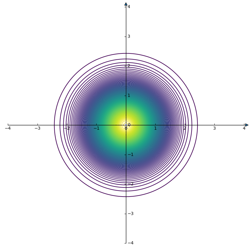
矩形:
import numpy as np
import matplotlib.pyplot as plt
import mpl_toolkits.axisartist as axisartist
from mpl_toolkits.mplot3d import Axes3D #画三维图不可少
from matplotlib import cm  #cm 是colormap的简写

#定义坐标轴函数
def setup_axes(fig, rect):
    ax = axisartist.Subplot(fig, rect)
    fig.add_axes(ax)

    ax.set_ylim(-4, 4)
    #自定义刻度
#    ax.set_yticks([-10, 0,9])
    ax.set_xlim(-4,4)
    ax.axis[:].set_visible(False)

	#第2条线,即y轴,经过x=0的点
    ax.axis["y"] = ax.new_floating_axis(1, 0)
    ax.axis["y"].set_axisline_style("-|>", size=1.5)
#    第一条线,x轴,经过y=0的点
    ax.axis["x"] = ax.new_floating_axis(0, 0)
    ax.axis["x"].set_axisline_style("-|>", size=1.5)

    return(ax)
# 1_dimension gaussian function
def gaussian(x,mu,sigma):
    f_x = 1/(sigma*np.sqrt(2*np.pi))*np.exp(-np.power(x-mu, 2.)/(2*np.power(sigma,2.)))
    return(f_x)

# 2_dimension gaussian function
def gaussian_2(x,y,mu_x,mu_y,sigma_x,sigma_y):
    f_x_y = 1/(sigma_x*sigma_y*(np.sqrt(2*np.pi))**2)*np.exp(-np.power\
              (x-mu_x, 2.)/(2*np.power(sigma_x,2.))-np.power(y-mu_y, 2.)/\
              (2*np.power(sigma_y,2.)))
    return(f_x_y)

#设置画布
fig = plt.figure(figsize=(8, 8)) #建议可以直接plt.figure()不定义大小
ax1 = setup_axes(fig, 111)
ax1.axis["x"].set_axis_direction("bottom")
ax1.axis[''y''].set_axis_direction(''right'')
# #在已经定义好的画布上加入高斯函数
x_values = np.linspace(-5,5,2000)
y_values = np.linspace(-5,5,2000)
X,Y = np.meshgrid(x_values,y_values)
mu_x,mu_y,sigma_x,sigma_y = 0,0,0.8,0.8
#F_x_y = gaussian_2(X,Y,mu_x,mu_y,sigma_x,sigma_y)
F_x_y = gaussian(X,mu_x,sigma_x)
#显示2d等高线图,画100条线
plt.contour(X,Y,F_x_y,100)
fig.show() 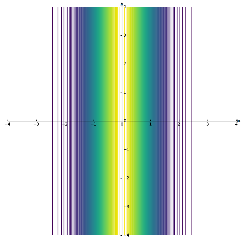
球
from mpl_toolkits.mplot3d import Axes3D
import matplotlib.pyplot as plt
import numpy as np
fig = plt.figure()
ax = fig.add_subplot(111, projection=''3d'')
u = np.linspace(0, 2 * np.pi, 100)
v = np.linspace(0, np.pi, 100)
x = 10 * np.outer(np.cos(u), np.sin(v))
y = 10 * np.outer(np.sin(u), np.sin(v))
z = 10 * np.outer(np.ones(np.size(u)), np.cos(v))
ax.plot_surface(x, y, z,  rstride=4, cstride=4, color=''b'')
plt.show()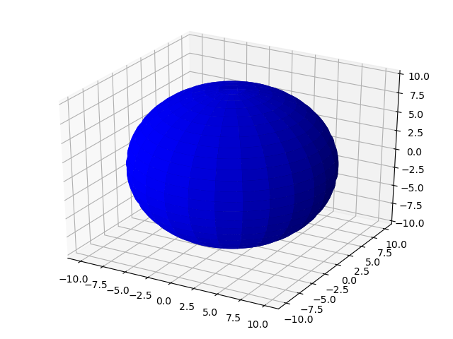
今天关于Python中的Gauss-Legendre算法和python legend的分享就到这里,希望大家有所收获,若想了解更多关于CPython 3.9 python.gram文件-尝试使用utf-8文本运行make regen-pegen时出错、openGauss数据库之Python驱动快速入门、PHP中的gmp_legendre()函数、python gaussian,gaussian2等相关知识,可以在本站进行查询。
本文标签:


