今天在找R shiny的教程的时候发现了一幅比较漂亮的散点图，配色很好看，代码记录在这里。

先贴出结果图，就是这样式的！

原文地址

https://www.r-bloggers.com/r-shiny-vs-tableau-3-business-application-examples/

作图代码

构造数据

data_apps<-data.frame(application=c("R Shiny","Python Dash","Excel","Tableau","PowerBI","Matlib","SAS"),
                      business_capability=c(10,8,4,6,5,6,7),
                      easy_of_learning=c(5,4,10,7,8,2,4),
                      trend=c(10,10,7,6,6,1,3),
                      cost=c("Free","Free","Low","Low","Low","High","High"))

加载需要的包

library(ggplot2)
library(ggrepel)
#install.packages("tidyquant")
library(tidyquant)

画图

ggplot(data_apps,aes(x=business_capability,y=easy_of_learning,
                     color=cost,size=trend))+
  geom_point()+
  geom_label_repel(aes(label=application,fill=application),
                   size=3.5,fontface="bold",color="white",
                   box.padding = 0.1,point.padding = 0.5,
                   segment.color = ''grey50'',segment.size = 1)+
  geom_smooth(color=palette_dark()[[1]],method = "lm",se=F,show.legend = F)+
  expand_limits(x=c(0,10),y=c(0,10))+
  theme_tq()+
  theme(legend.direction = "vertical",
        legend.position = "right",
        legend.title = element_text(size=8),
        legend.text = element_text(size=8))+
  scale_fill_tq()+
  scale_color_tq()+
  scale_y_continuous(breaks = seq(0, 10, 2)) +
  scale_x_continuous(breaks = 0:10) +
  scale_size_continuous(range = c(2, 14)) + 
  labs(title = "Dashboard and Business Application Tools",
       subtitle = "R has a longer learning curve but has a massive business capability rating",
       x     = "Business Capability Rating (10 = Powerful)",
       y     = "Learning Curve (10 = Easy to Learn)",
       color = "Cost",
       size  = "Trend",
       fill  = "Tool") 

tidyquant这个包时第一次使用，上面的代码中palette_dark()、theme_tq()、scale_fill_tq()、scale_color_tq()都是来自这个包中的函数。

使用help(package="tidyquant")查看帮助文档 看到了一句话

Bringing financial and business analysis to the tidyverse

这个包应该是应用于金融领域的。

对于我来说可能是会用到这里的主题和配色方案！

接下来看一个帮助文档的例子https://business-science.github.io/tidyquant/reference/theme_tq.html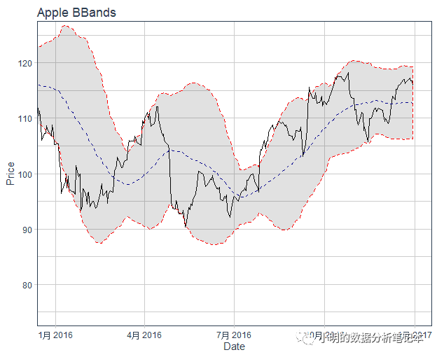

代码是

library(tidyquant)
library(dplyr)
library(ggplot2)

AAPL <- tq_get("AAPL", from = "2013-01-01", to = "2016-12-31")
AAPL
write.csv(AAPL,file="AAPL.csv",row.names = F,quote = F)

AAPL %>% ggplot(aes(x = date, y = close)) +
  geom_line() +
  geom_bbands(aes(high = high, low = low, close = close),
              ma_fun = EMA,
              wilder = TRUE,
              ratio = NULL,
              n = 50) +
  coord_x_date(xlim = c("2016-01-01", "2016-12-31"),
               ylim = c(75, 125)) +
  labs(title = "Apple BBands",
       x = "Date",
       y = "Price") +
  theme_tq()

重复这个例子获取数据可能需要科学上网，需要这个数据集的可以给我的公众号留言！

还用一个函数是palette_dark()包括12个颜色 画个柱形图看一下

df<-data.frame(x=LETTERS[1:12],y=1:12)

x1<-palette_dark()
matrix(x1)[,1]
p1<-ggplot(df,aes(x,y))+
  geom_col(aes(fill=x))+
  theme_bw()+
  scale_fill_manual(values = matrix(x1)[,1])+
  ggtitle("palette_dark()")+
  labs(x="",y="")+
  theme(legend.position = "none")
x2<-palette_green()
p2<-ggplot(df,aes(x,y))+
  geom_col(aes(fill=x))+
  theme_bw()+
  scale_fill_manual(values = matrix(x2)[,1])+
  ggtitle("palette_green()")+
  labs(x="",y="")+
  theme(legend.position = "none")
x3<-palette_light()
p3<-ggplot(df,aes(x,y))+
  geom_col(aes(fill=x))+
  theme_bw()+
  scale_fill_manual(values = matrix(x3)[,1])+
  ggtitle("palette_light()")+
  labs(x="",y="")+
  theme(legend.position = "none")
cowplot::plot_grid(p1,p2,p3,ncol=1,align = "v")

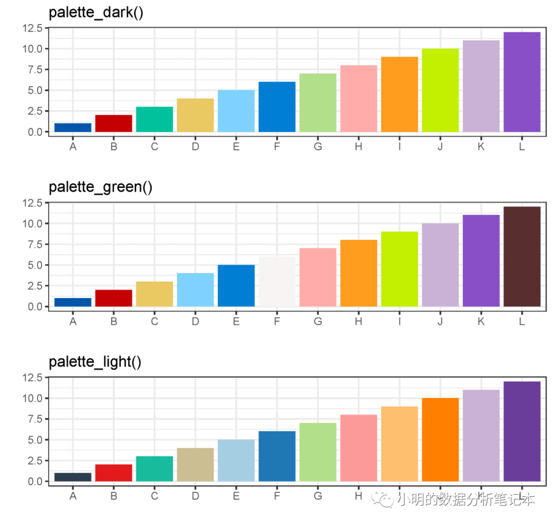
这个配色很好看！可以作为备选！ 这三个函数产生的颜色好像是一样的，只是顺序不一样！

欢迎大家关注我的公众号

小明的数据分析笔记本