想了解Tensorflow:如何替换计算图中的节点?的新动态吗?本文将为您提供详细的信息,我们还将为您解答关于tensorflow修改模型结构的相关问题,此外,我们还将为您介绍关于130、Tensor
想了解Tensorflow:如何替换计算图中的节点?的新动态吗?本文将为您提供详细的信息,我们还将为您解答关于tensorflow修改模型结构的相关问题,此外,我们还将为您介绍关于130、TensorFlow 操作多个计算图、Python-Tensorflow:如何保存/恢复模型?、SSD-Tensorflow: 3 步运行 TensorFlow 单图片多盒目标检测器、Tensorboard 教程:Tensorflow 命名空间与计算图可视化的新知识。
本文目录一览:- Tensorflow:如何替换计算图中的节点?(tensorflow修改模型结构)
- 130、TensorFlow 操作多个计算图
- Python-Tensorflow:如何保存/恢复模型?
- SSD-Tensorflow: 3 步运行 TensorFlow 单图片多盒目标检测器
- Tensorboard 教程:Tensorflow 命名空间与计算图可视化
")
Tensorflow:如何替换计算图中的节点?(tensorflow修改模型结构)
如果您有两个不相交的图,并且想要链接它们,请执行以下操作:
x = tf.placeholder(''float'')y = f(x)y = tf.placeholder(''float'')z = f(y)到这个:
x = tf.placeholder(''float'')y = f(x)z = g(y)有没有办法做到这一点?在某些情况下,这似乎可以使施工更容易。
例如,如果您有一个图,其输入图像为tf.placeholder,并且想要优化输入图像(深梦风格),是否有一种方法可以仅用tf.variable节点替换占位符?还是在构建图形之前必须考虑一下?
答案1
小编典典TL;
DR:如果可以将这两个计算定义为Python函数,则应该这样做。如果不能,那么TensorFlow中有更多高级功能可用于序列化和导入图形,这使您可以从不同来源组成图形。
在TensorFlow中执行此操作的一种方法是将不相交的计算构建为单独的tf.Graph对象,然后使用以下命令将它们转换为序列化的协议缓冲区Graph.as_graph_def():
with tf.Graph().as_default() as g_1: input = tf.placeholder(tf.float32, name="input") y = f(input) # NOTE: using identity to get a known name for the output tensor. output = tf.identity(y, name="output")gdef_1 = g_1.as_graph_def()with tf.Graph().as_default() as g_2: # NOTE: g_2 not g_1 input = tf.placeholder(tf.float32, name="input") z = g(input) output = tf.identity(y, name="output")gdef_2 = g_2.as_graph_def()然后,你可以撰写gdef_1和gdef_2成第三曲线,使用tf.import_graph_def():
with tf.Graph().as_default() as g_combined: x = tf.placeholder(tf.float32, name="") # Import gdef_1, which performs f(x). # "input:0" and "output:0" are the names of tensors in gdef_1. y, = tf.import_graph_def(gdef_1, input_map={"input:0": x}, return_elements=["output:0"]) # Import gdef_2, which performs g(y) z, = tf.import_graph_def(gdef_2, input_map={"input:0": y}, return_elements=["output:0"]
130、TensorFlow 操作多个计算图
# Programming with multiple graphs
# 当训练一个模型的时候一个常用的方式就是使用一个图来训练你的模型
# 另一个图来评价和计算训练的效果
# 在许多情况下前向计算和训练是不同的
# 例如像Dropout和batch正则化使用不同的操作在不同的Case条件下
# 更进一步地说 通过使用默认的工具类,如tf.train.Saver使用tf.Variable的命名空间
# 在保存检查点的时候tf.Variable的名字是根据tf.Operation来定义
# 当你使用这种方法来编程的时候你或者使用独立的Python进程来建立和执行这个计算图
# 或者你可以使用多个计算图在相同的进程中
# tf.Graph为tf.Operation定义了命名空间
# 每一个操作必须有唯一的名字
# TensorFlow会通过在操作名字后面appending上_1,_2
# 如果所起的名字已经存在了,使用多个计算图能够让你更好地控制每个计算节点

# 默认的图存储信息关于每个tf.Operation和tf.Tensor
# 如果你对程序创建了更大数量的没有被连接的子图
# 使用多个计算图或许是更有效果的。因此, 不相关的状态可以被垃圾收集
import tensorflow as tf
g_1 = tf.Graph()
with g_1.as_default():
    # Operations created in this scope will be added to ''g_1''
    c = tf.constant("Node in g_1")

    # Sessions created in this scope will run operations from ''g_1''
    sess_1 = tf.Session()
g_2 = tf.Graph()
with g_2.as_default():
    # operations created in this scope will be added to ''g_2''
    d = tf.constant("Node in g_2")

# Alternatively , you can pass a graph when constructing a ''tf.Session''
# ''sess_2'' will run operations from ''g_2''
sess_2 = tf.Session(graph=g_2)
assert c.graph is g_1
assert sess_1.graph is g_1

assert d.graph is g_2
assert sess_2.graph is g_2

Python-Tensorflow:如何保存/恢复模型?
如何解决Python-Tensorflow:如何保存/恢复模型??
从文档:
保存
# Create some variables.
v1 = tf.get_variable("v1", shape=[3], initializer = tf.zeros_initializer)
v2 = tf.get_variable("v2", shape=[5], initializer = tf.zeros_initializer)

inc_v1 = v1.assign(v1+1)
dec_v2 = v2.assign(v2-1)

# Add an op to initialize the variables.
init_op = tf.global_variables_initializer()

# Add ops to save and restore all the variables.
saver = tf.train.Saver()

# Later, launch the model, initialize the variables, do some work, and save the
# variables to disk.
with tf.Session() as sess:
  sess.run(init_op)
  # Do some work with the model.
  inc_v1.op.run()
  dec_v2.op.run()
  # Save the variables to disk.
  save_path = saver.save(sess, "/tmp/model.ckpt")
  print("Model saved in path: %s" % save_path)
恢复
tf.reset_default_graph()

# Create some variables.
v1 = tf.get_variable("v1", shape=[3])
v2 = tf.get_variable("v2", shape=[5])

# Add ops to save and restore all the variables.
saver = tf.train.Saver()

# Later, launch the model, use the saver to restore variables from disk, and
# do some work with the model.
with tf.Session() as sess:
  # Restore variables from disk.
  saver.restore(sess, "/tmp/model.ckpt")
  print("Model restored.")
  # Check the values of the variables
  print("v1 : %s" % v1.eval())
  print("v2 : %s" % v2.eval())
Tensorflow 2
这仍然是测试版,因此我建议不要使用。如果你仍然想走那条路,这里是tf.saved_model使用指南
为了完整起见,我给出了很多好答案,我将加2美分:simple_save。也是使用tf.data.DatasetAPI 的独立代码示例。
Python 3; Tensorflow 1.14

import tensorflow as tf
from tensorflow.saved_model import tag_constants

with tf.Graph().as_default():
    with tf.Session() as sess:
        ...

        # Saving
        inputs = {
            "batch_size_placeholder": batch_size_placeholder,
            "features_placeholder": features_placeholder,
            "labels_placeholder": labels_placeholder,
        }
        outputs = {"prediction": model_output}
        tf.saved_model.simple_save(
            sess, ''path/to/your/location/'', inputs, outputs
        )
恢复:
graph = tf.Graph()
with restored_graph.as_default():
    with tf.Session() as sess:
        tf.saved_model.loader.load(
            sess,
            [tag_constants.SERVING],
            ''path/to/your/location/'',
        )
        batch_size_placeholder = graph.get_tensor_by_name(''batch_size_placeholder:0'')
        features_placeholder = graph.get_tensor_by_name(''features_placeholder:0'')
        labels_placeholder = graph.get_tensor_by_name(''labels_placeholder:0'')
        prediction = restored_graph.get_tensor_by_name(''dense/BiasAdd:0'')

        sess.run(prediction, Feed_dict={
            batch_size_placeholder: some_value,
            features_placeholder: some_other_value,
            labels_placeholder: another_value
        })
为了演示,以下代码生成随机数据。
- 我们首先创建占位符。它们将在运行时保存数据。根据它们,我们创建
Dataset,然后创建Iterator。我们得到迭代器的生成张量,称为input_tensor,它将用作模型的输入。 - 该模型本身是
input_tensor基于:基于GRU的双向RNN,然后是密集分类器。因为为什么不。 - 损耗为
softmax_cross_entropy_with_logits,优化为Adam。经过2个时期(每个批次2个批次)后,我们使用保存了“训练”模型tf.saved_model.simple_save。如果按原样运行代码,则模型将保存在simple/当前工作目录下的文件夹中。 - 在新图形中,然后使用还原保存的模型
tf.saved_model.loader.load。我们使用捕获占位符并登录,graph.get_tensor_by_name并使用进行Iterator初始化操作graph.get_operation_by_name。 - 最后,我们对数据集中的两个批次进行推断,并检查保存和恢复的模型是否产生相同的值。他们是这样! 代码:
import os
import shutil
import numpy as np
import tensorflow as tf
from tensorflow.python.saved_model import tag_constants


def model(graph, input_tensor):
    """Create the model which consists of
    a bidirectional rnn (GRU(10)) followed by a dense classifier

    Args:
        graph (tf.Graph): Tensors'' graph
        input_tensor (tf.Tensor): Tensor fed as input to the model

    Returns:
        tf.Tensor: the model''s output layer Tensor
    """
    cell = tf.nn.rnn_cell.GRUCell(10)
    with graph.as_default():
        ((fw_outputs, bw_outputs), (fw_state, bw_state)) = tf.nn.bidirectional_dynamic_rnn(
            cell_fw=cell,
            cell_bw=cell,
            inputs=input_tensor,
            sequence_length=[10] * 32,
            dtype=tf.float32,
            swap_memory=True,
            scope=None)
        outputs = tf.concat((fw_outputs, bw_outputs), 2)
        mean = tf.reduce_mean(outputs, axis=1)
        dense = tf.layers.dense(mean, 5, activation=None)

        return dense


def get_opt_op(graph, logits, labels_tensor):
    """Create optimization operation from model''s logits and labels

    Args:
        graph (tf.Graph): Tensors'' graph
        logits (tf.Tensor): The model''s output without activation
        labels_tensor (tf.Tensor): Target labels

    Returns:
        tf.Operation: the operation performing a stem of Adam optimizer
    """
    with graph.as_default():
        with tf.variable_scope(''loss''):
            loss = tf.reduce_mean(tf.nn.softmax_cross_entropy_with_logits(
                    logits=logits, labels=labels_tensor, name=''xent''),
                    name="mean-xent"
                    )
        with tf.variable_scope(''optimizer''):
            opt_op = tf.train.AdamOptimizer(1e-2).minimize(loss)
        return opt_op


if __name__ == ''__main__'':
    # Set random seed for reproducibility
    # and create synthetic data
    np.random.seed(0)
    features = np.random.randn(64, 10, 30)
    labels = np.eye(5)[np.random.randint(0, 5, (64,))]

    graph1 = tf.Graph()
    with graph1.as_default():
        # Random seed for reproducibility
        tf.set_random_seed(0)
        # Placeholders
        batch_size_ph = tf.placeholder(tf.int64, name=''batch_size_ph'')
        features_data_ph = tf.placeholder(tf.float32, [None, None, 30], ''features_data_ph'')
        labels_data_ph = tf.placeholder(tf.int32, [None, 5], ''labels_data_ph'')
        # Dataset
        dataset = tf.data.Dataset.from_tensor_slices((features_data_ph, labels_data_ph))
        dataset = dataset.batch(batch_size_ph)
        iterator = tf.data.Iterator.from_structure(dataset.output_types, dataset.output_shapes)
        dataset_init_op = iterator.make_initializer(dataset, name=''dataset_init'')
        input_tensor, labels_tensor = iterator.get_next()

        # Model
        logits = model(graph1, input_tensor)
        # Optimization
        opt_op = get_opt_op(graph1, logits, labels_tensor)

        with tf.Session(graph=graph1) as sess:
            # Initialize variables
            tf.global_variables_initializer().run(session=sess)
            for epoch in range(3):
                batch = 0
                # Initialize dataset (Could Feed epochs in Dataset.repeat(epochs))
                sess.run(
                    dataset_init_op,
                    Feed_dict={
                        features_data_ph: features,
                        labels_data_ph: labels,
                        batch_size_ph: 32
                    })
                values = []
                while True:
                    try:
                        if epoch < 2:
                            # Training
                            _, value = sess.run([opt_op, logits])
                            print(''Epoch {}, batch {} | Sample value: {}''.format(epoch, batch, value[0]))
                            batch += 1
                        else:
                            # Final inference
                            values.append(sess.run(logits))
                            print(''Epoch {}, batch {} | Final inference | Sample value: {}''.format(epoch, batch, values[-1][0]))
                            batch += 1
                    except tf.errors.OutOfRangeError:
                        break
            # Save model state
            print(''\nSaving...'')
            cwd = os.getcwd()
            path = os.path.join(cwd, ''simple'')
            shutil.rmtree(path, ignore_errors=True)
            inputs_dict = {
                "batch_size_ph": batch_size_ph,
                "features_data_ph": features_data_ph,
                "labels_data_ph": labels_data_ph
            }
            outputs_dict = {
                "logits": logits
            }
            tf.saved_model.simple_save(
                sess, path, inputs_dict, outputs_dict
            )
            print(''Ok'')
    # Restoring
    graph2 = tf.Graph()
    with graph2.as_default():
        with tf.Session(graph=graph2) as sess:
            # Restore saved values
            print(''\nRestoring...'')
            tf.saved_model.loader.load(
                sess,
                [tag_constants.SERVING],
                path
            )
            print(''Ok'')
            # Get restored placeholders
            labels_data_ph = graph2.get_tensor_by_name(''labels_data_ph:0'')
            features_data_ph = graph2.get_tensor_by_name(''features_data_ph:0'')
            batch_size_ph = graph2.get_tensor_by_name(''batch_size_ph:0'')
            # Get restored model output
            restored_logits = graph2.get_tensor_by_name(''dense/BiasAdd:0'')
            # Get dataset initializing operation
            dataset_init_op = graph2.get_operation_by_name(''dataset_init'')

            # Initialize restored dataset
            sess.run(
                dataset_init_op,
                Feed_dict={
                    features_data_ph: features,
                    labels_data_ph: labels,
                    batch_size_ph: 32
                }

            )
            # Compute inference for both batches in dataset
            restored_values = []
            for i in range(2):
                restored_values.append(sess.run(restored_logits))
                print(''Restored values: '', restored_values[i][0])

    # Check if original inference and restored inference are equal
    valid = all((v == rv).all() for v, rv in zip(values, restored_values))
    print(''\nInferences match: '', valid)
这将打印:
$ python3 save_and_restore.py

Epoch 0, batch 0 | Sample value: [-0.13851789 -0.3087595   0.12804556  0.20013677 -0.08229901]
Epoch 0, batch 1 | Sample value: [-0.00555491 -0.04339041 -0.05111827 -0.2480045  -0.00107776]
Epoch 1, batch 0 | Sample value: [-0.19321944 -0.2104792  -0.00602257  0.07465433  0.11674127]
Epoch 1, batch 1 | Sample value: [-0.05275984  0.05981954 -0.15913513 -0.3244143   0.10673307]
Epoch 2, batch 0 | Final inference | Sample value: [-0.26331693 -0.13013336 -0.12553    -0.04276478  0.2933622 ]
Epoch 2, batch 1 | Final inference | Sample value: [-0.07730117  0.11119192 -0.20817074 -0.35660955  0.16990358]

Saving...
INFO:tensorflow:Assets added to graph.
INFO:tensorflow:No assets to write.
INFO:tensorflow:SavedModel written to: b''/some/path/simple/saved_model.pb''
Ok

Restoring...
INFO:tensorflow:Restoring parameters from b''/some/path/simple/variables/variables''
Ok
Restored values:  [-0.26331693 -0.13013336 -0.12553    -0.04276478  0.2933622 ]
Restored values:  [-0.07730117  0.11119192 -0.20817074 -0.35660955  0.16990358]

Inferences match:  True
解决方法
在Tensorflow中训练模型后:
你如何保存经过训练的模型?
以后如何恢复此保存的模型?

SSD-Tensorflow: 3 步运行 TensorFlow 单图片多盒目标检测器
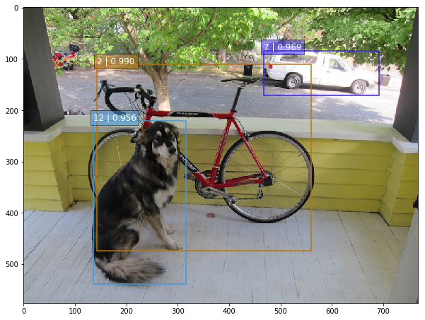
昨天类似的 YOLO: https://www.v2ex.com/t/392671#reply0
下载这个项目
https://github.com/balancap/SSD-Tensorflow
解压 checkpoint files in ./checkpoint
unzip ssd_300_vgg.ckpt.zip
运行 jupyter 文件命令
jupyter notebook notebooks/ssd_notebook.ipynb
项目说明: http://www.tensorflownews.com/2017/09/22/ssd-single-shot-multibox-detector-in-tensorflow/
项目地址: https://github.com/balancap/SSD-Tensorflow
更多 TensorFlow 教程: http://www.tensorflownews.com

Tensorboard 教程:Tensorflow 命名空间与计算图可视化
Tensorflow 命名空间与计算图可视化
觉得有用的话,欢迎一起讨论相互学习~Follow Me
参考文献 强烈推荐 Tensorflow 实战 Google 深度学习框架 实验平台: Tensorflow1.4.0 python3.5.0
- Tensorflow 可视化得到的图并不仅是将 Tensorflow 计算图中的节点和边直接可视化,它会根据每个 Tensorflow 计算节点的命名空间来整理可视化得到效果图,使得神经网络的整体结构不会被过多的细节所淹没。除了显示 Tensorflow 计算图的结构,Tensorflow 还可以展示 Tensorflow 计算节点上的信息进行描述统计,包括频数统计和分布统计。
- 为了更好的组织可视化效果图中的计算节点,Tensorboard 支持通过 Tensorflow 命名空间来整理可视化效果图上的节点。在 Tensorboard 的默认视图中,Tensorflow 计算图中同一个命名空间下的所有节点会被缩略为一个节点,而顶层命名空间的节点才会被显示在 Tensorboard 可视化效果图中。
<font color=Purple>tf.variable_scope 和 tf.name_scope 函数区别 </font>
- tf.variable_scope 和 tf.name_scope 函数都提供了命名变量管理的功能,这两个函数在大部分情况下是等价的,唯一的区别在于使用 tf.get_variable 函数时:
import tensorflow as tf
# 不同的命名空间
with tf.variable_scope("foo"):
    # 在命名空间foo下获取变量"bar",于是得到的变量名称为"foo/bar"
    a = tf.get_variable("bar", [1])
    print(a.name)
    # foo/bar:0
with tf.variable_scope("bar"):
    # 在命名空间bar下获取变量"bar",于是得到的变量名称为"bar/bar".此时变量在"bar/bar"和变量"foo/bar"并不冲突,于是可以正常运行
    b = tf.get_variable("bar", [1])
    print(b.name)
    # bar/bar:0
#  tf.Variable和tf.get_variable的区别。

with tf.name_scope("a"):
    # 使用tf.Variable函数生成变量时会受到tf.name_scope影响,于是这个变量的名称为"a/Variable"
    a = tf.Variable([1])
    print(a.name)
    # a/Variable: 0

    # tf.get_variable函数不受头tf.name_scope函数的影响,于是变量并不在a这个命名空间中
    a = tf.get_variable("b", [1])
    print(a.name)
    # b:0

# with tf.name_scope("b"):
    # 因为tf.get_variable不受tf.name_scope影响,所以这里将试图获取名称为"a"的变量。然而这个变量已经被声明了,于是这里会报重复声明的错误。
    # tf.get_variable("b",[1])
- 通过对变量命名空间进行管理,使用 Tensorboard 查看模型的结构时更加清晰
import tensorflow as tf
with tf.name_scope("input1"):
    input1 = tf.constant([1.0, 2.0, 3.0], name="input2")
with tf.name_scope("input2"):
    input2 = tf.Variable(tf.random_uniform([3]), name="input2")
output = tf.add_n([input1, input2], name="add")

writer = tf.summary.FileWriter("log/simple_example.log", tf.get_default_graph())
writer.close()
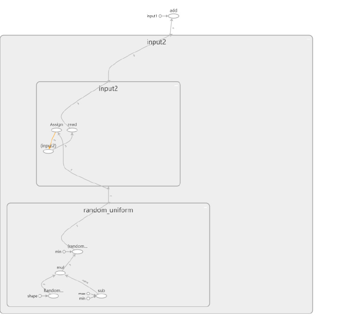
- 这样程序中定义的加法运算都被清晰的展示出来,并且变量初始化等基本操作都被折叠起来。
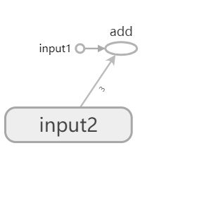
- 点击 input2 上的加号按钮,能够看到关于 input2 变量初始化的全过程。
<font color=Purple> 可视化 MNIST 程序 </font>
MNIST 基本程序
import tensorflow as tf
from tensorflow.examples.tutorials.mnist import input_data
# mnist_inference中定义的常量和前向传播的函数不需要改变,因为前向传播已经通过
# tf.variable_scope实现了计算节点按照网络结构的划分
import mnist_inference

# #### 1. 定义神经网络的参数。
BATCH_SIZE = 100
LEARNING_RATE_BASE = 0.8
LEARNING_RATE_DECAY = 0.99
REGULARIZATION_RATE = 0.0001
TRAINING_STEPS = 3000
MOVING_AVERAGE_DECAY = 0.99


# #### 2. 定义训练的过程并保存TensorBoard的log文件。
def train(mnist):
    #  将处理输入数据的计算都放在名字为"input"的命名空间中
    with tf.name_scope(''input''):
        x = tf.placeholder(tf.float32, [None, mnist_inference.INPUT_NODE], name=''x-input'')
        y_ = tf.placeholder(tf.float32, [None, mnist_inference.OUTPUT_NODE], name=''y-input'')
    regularizer = tf.contrib.layers.l2_regularizer(REGULARIZATION_RATE)
    y = mnist_inference.inference(x, regularizer)
    global_step = tf.Variable(0, trainable=False)

    # 将处理滑动平均相关的计算都放在名为moving average 的命名空间下。
    with tf.name_scope("moving_average"):
        variable_averages = tf.train.ExponentialMovingAverage(MOVING_AVERAGE_DECAY, global_step)
        variables_averages_op = variable_averages.apply(tf.trainable_variables())  # 对可训练变量集合使用滑动平均

    # 将计算损失函数相关的计算都放在名为loss function 的命名空间下。
    with tf.name_scope("loss_function"):
        cross_entropy = tf.nn.sparse_softmax_cross_entropy_with_logits(logits=y, labels=tf.argmax(y_, 1))
        cross_entropy_mean = tf.reduce_mean(cross_entropy)
        # 将交叉熵加上权值的正则化
        loss = cross_entropy_mean + tf.add_n(tf.get_collection(''losses''))

    # 将定义学习率、优化方法以及每一轮训练需要执行的操作都放在名字为"train_step"的命名空间下。
    with tf.name_scope("train_step"):
        learning_rate = tf.train.exponential_decay(
            LEARNING_RATE_BASE,
            global_step,
            mnist.train.num_examples/BATCH_SIZE, LEARNING_RATE_DECAY,
            staircase=True)

        train_step = tf.train.GradientDescentOptimizer(learning_rate).minimize(loss, global_step=global_step)
        # 在反向传播的过程中更新变量的滑动平均值
        with tf.control_dependencies([train_step, variables_averages_op]):
            train_op = tf.no_op(name=''train'')
    # 将结果记录进log文件夹中
    writer = tf.summary.FileWriter("log", tf.get_default_graph())

    # 训练模型。
    with tf.Session() as sess:
        tf.global_variables_initializer().run()
        for i in range(TRAINING_STEPS):
            xs, ys = mnist.train.next_batch(BATCH_SIZE)

            if i%1000 == 0:
                # 配置运行时需要记录的信息。
                run_options = tf.RunOptions(trace_level=tf.RunOptions.FULL_TRACE)
                # 运行时记录运行信息的proto。
                run_metadata = tf.RunMetadata()
                # 将配置信息和记录运行信息的proto传入运行的过程,从而记录运行时每一个节点的时间空间开销信息
                _, loss_value, step = sess.run(
                    [train_op, loss, global_step], feed_dict={x: xs, y_: ys},
                    options=run_options, run_metadata=run_metadata)
                writer.add_run_metadata(run_metadata=run_metadata, tag=("tag%d"%i), global_step=i)
                print("After %d training step(s), loss on training batch is %g."%(step, loss_value))
            else:
                _, loss_value, step = sess.run([train_op, loss, global_step], feed_dict={x: xs, y_: ys})

    writer.close()


# #### 3. 主函数。
def main(argv=None):
    mnist = input_data.read_data_sets("../../datasets/MNIST_data", one_hot=True)
    train(mnist)


if __name__ == ''__main__'':
    main()
<font color=DeepPink> 可视化效果图 </font>
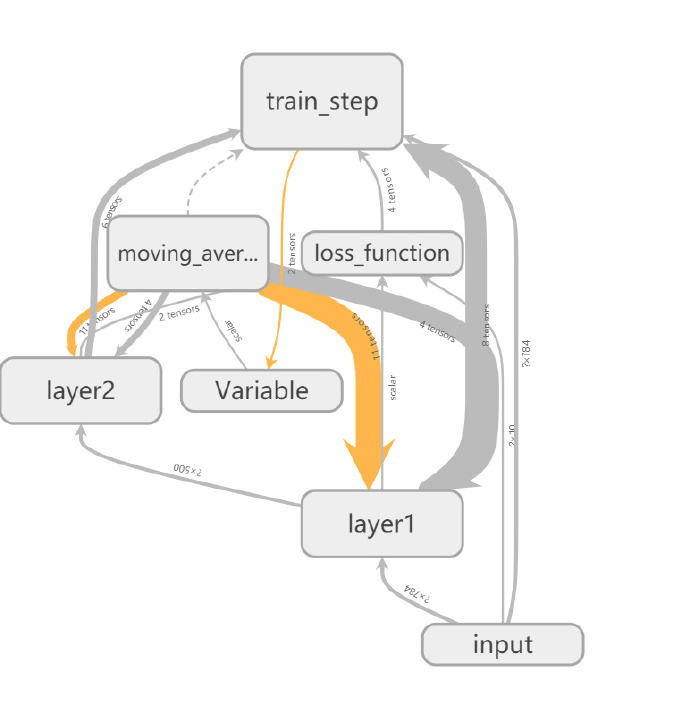
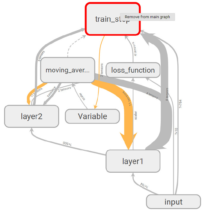
- input 节点代表了训练神经网络需要的输入数据,这些输入数据会提供给神经网络的第一层 layer1. 然后神经网络第一层 layerl 的结果会被传到第二层 layer2, 经过 layer2 的计算得到前向传播的结果.loss function 节点表示计算损失函数的过程,这个过程既依赖于前向传播的结果来计算交叉熵 (layer2 到 loss_function 的边,又依赖于每一层中所定义的变量来计算 L2 正则化损失 (layer1 和 layer2 到 loss_function 的边).loss_function 的计算结果会提供给神经网络的优化过程,也就是图中位 train_step 所代表的节点。
- 发现节点之间有两种不同的边。一种边是通过实线表示的,这种边刻画了数据传输,边上箭头方向表达了数据传输的方向。比如 layerl 和 layer2 之间的边表示了 layer1 的输出将会作为 layer2 的输入。TensorBoard 可视化效果图的边上还标注了张量的维度信息。
- 从图中可以看出,节点 input 和 layer1 之间传输的张量的维度为 * 784。这说明了训练时提供的 batch 大小不是固定的(也就是定义的时候是 None),输入层节点的个数为 784。当两个节点之间传输的张量多于 1 时,可视化效果图上将只显示张量的个数。效果图上边的粗细表示的是两个节点之间传输的标量维度的总大小,而不是传输的标量个数。比如 layer2 和 train_step 之间虽然传输了 6 个张量,但其维度都比较小,所以这条边比 layerl 和 moving_average 之间的边(只传输了 4 个张量〉还要细。当张量的维度无法确定时,TensorBoard 会使用最细的边来表示。比如 layer1 与 layer2 之间的边。
- Tensor Board 可视化效果图上另外一种边是通过虚线表示的,比如图中所示的 moving_ average 和 train_step 之间的边。虚边表达了计算之间的依赖关系,比如在程序中,通过 tf.control_dependencies 函数指定了更新参数滑动平均值的操作和通过反向传播更新变量的操作需要同时进行,于是 moving_average 与 train_step 之间存在一条虚边.
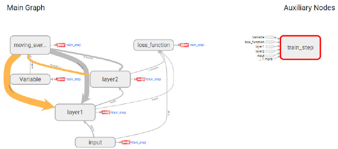
- 除了手动的通过 TensorFlow 中的命名空间来调整 TensorBoard 的可视化效果图,TensorBoard 也会智能地调整可视化效果图上的节点.TensorFlow 中部分计算节点会有比较多的依赖关系,如果全部画在一张图上会便可视化得到的效果图非常拥挤。于是 TensorBoard 将 TensorFlow 计算图分成了主图 (Main Graph) 和辅助图 (Auxiliary nodes) 两个部分来呈现。TensorBoard 会自动将连接比较多的节点放在辅助图中,使得主图的结构更加清晰。
- 除了自动的方式,TensorBoard 也支持手工的方式来调整可视化结果。右键单击可视化效果图上的节点会弹出一个选项,这个选项可以将节点加入主图或者从主图中删除。左键选择一个节点并点击信息框下部的选项也可以完成类似的功能。注意 TensorBoard 不会保存用户对计算图可视化结果的手工修改,页面刷新之后计算图可视化结果又会回到最初的样子。
今天关于Tensorflow:如何替换计算图中的节点?和tensorflow修改模型结构的分享就到这里,希望大家有所收获,若想了解更多关于130、TensorFlow 操作多个计算图、Python-Tensorflow:如何保存/恢复模型?、SSD-Tensorflow: 3 步运行 TensorFlow 单图片多盒目标检测器、Tensorboard 教程:Tensorflow 命名空间与计算图可视化等相关知识,可以在本站进行查询。
本文标签:


