想了解neuralink主要从事什么开发的新动态吗？本文将为您提供详细的信息，我们还将为您解答关于neuralink公司的相关问题，此外，我们还将为您介绍关于ArtificialNeuronsandS

想了解neuralink主要从事什么开发的新动态吗？本文将为您提供详细的信息，我们还将为您解答关于neuralink公司的相关问题，此外，我们还将为您介绍关于Artificial Neurons and Single-Layer Neural Networks、Bilinear CNN与 Randomly Wired Neural Network、EfficientNet: Rethinking Model Scaling for Convolutional Neural Networks、GBase8a数据库dblink主要使用场景介绍的新知识。

• neuralink主要从事什么开发（neuralink公司）
• Artificial Neurons and Single-Layer Neural Networks
• Bilinear CNN与 Randomly Wired Neural Network
• EfficientNet: Rethinking Model Scaling for Convolutional Neural Networks
• GBase8a数据库dblink主要使用场景介绍

neuralink主要从事什么开发（neuralink公司）

neuralink是一家美国的科技公司，许多人对其开发的研究对象都不太了解，这家公司主要研究方向是神经织网，这里就给大家简单介绍一下具体的操作方法。

neuralink主要从事什么开发

答： Neuralink是马斯克的创业公司，注册成立于2016年。

该公司专注于高带宽侵入式脑机接口技术，旨在将大脑和网络相连通。

据悉，现有的脑机接口一般分为侵入式和非侵入式接口，Neuralink

的研究一般属于前者。

通过在大脑中植入微小的电极，利用电流让计算机和脑细胞产生“互动”。

neuralink扩展阅读：

1、 这种设备一旦植入人脑，计算机便可以把一个人的想法转化为行动，

让人们只需在大脑中想到某个行为，计算机便可执行诸如打字和按下按钮之类的操作。

2、Neuralink成立之初，马斯克曾探讨过一个科幻小说的概念——神经织网 (neural lace)

一个无缝、稳定、可以直接与大脑通信的全脑接口。据马斯克透露，

Neuralink设备有朝一日能实现“人工智能共生” (AI symbiosis) ，即人脑将和人工智能融合。

3、Neuralink的工作内容可以概括为一点：他们试图研发一种技术，将人脑与计算机系统融合在一起。

这种利用脑机接口实现的融合，将有助于治疗人类的脑部疾病。以及，很可能，使人类变得更加强大。

相关阅读：是什么意思

Artificial Neurons and Single-Layer Neural Networks

In [1]:

import sys
sys.path = [''/Users/sebastian/github/mlxtend/''] + sys.path

In [2]:

%load_ext watermark
%watermark -a ''Sebastian Raschka'' -v

Sebastian Raschka 

CPython 3.4.3
IPython 3.0.0

Artificial Neurons and Single-Layer Neural Networks

- How Machine Learning Algorithms Work Part 1

This article offers a brief glimpse of the history and basic concepts of machine learning. We will take a look at the first algorithmically described neural network and the gradient descent algorithm in context of adaptive linear neurons, which will not only introduce the principles of machine learning but also serve as the basis for modern multilayer neural networks in future articles.

Sections

• Introduction
• Artificial Neurons and the McCulloch-Pitts Model
• Frank Rosenblatt''s Perceptron
  • The Unit Step Function
  • The Perceptron Learning Rule
  • Implementing the Perceptron Rule in Python
  • Problems with Perceptrons
• Adaptive Linear Neurons and the Delta Rule
  • Gradient Descent
  • The Gradient Descent Rule in Action
  • Online Learning via Stochastic Gradient Descent
• What''s Next?
• References

Introduction

[back to top]

Machine learning is one of the hottest and most exciting fields in the modern age of technology. Thanks to machine learning, we enjoy robust email spam filters, convenient text and voice recognition, reliable web search engines, challenging chess players, and, hopefully soon, safe and efficient self-driving cars.

Without any doubt, machine learning has become a big and popular field, and sometimes it may be challenging to see the (random) forest for the (decision) trees. Thus, I thought that it might be worthwhile to explore different machine learning algorithms in more detail by not only discussing the theory but also by implementing them step by step.

To briefly summarize what machine learning is all about: "[Machine learning is the] field of study that gives computers the ability to learn without being explicitly programmed" (Arthur Samuel, 1959). Machine learning is about the development and use of algorithms that can recognize patterns in data in order to make decisions based on statistics, probability theory, combinatorics, and optimization.

The first article in this series will introduce perceptrons and the adaline (ADAptive LINear NEuron), which fall into the category of single-layer neural networks. The perceptron is not only the first algorithmically described learning algorithm [1], but it is also very intuitive, easy to implement, and a good entry point to the (re-discovered) modern state-of-the-art machine learning algorithms: Artificial neural networks (or "deep learning" if you like). As we will see later, the adaline is a consequent improvement of the perceptron algorithm and offers a good opportunity to learn about a popular optimization algorithm in machine learning: gradient descent.

Artificial Neurons and the McCulloch-Pitts Model

[back to top]

The initial idea of the perceptron dates back to the work of Warren McCulloch and Walter Pitts in 1943 [2], who drew an analogy between biological neurons and simple logic gates with binary outputs. In more intuitive terms, neurons can be understood as the subunits of a neural network in a biological brain. Here, the signals of variable magnitudes arrive at the dendrites. Those input signals are then accumulated in the cell body of the neuron, and if the accumulated signal exceeds a certain threshold, a output signal is generated that which will be passed on by the axon.

Frank Rosenblatt''s Perceptron

[back to top]

To continue with the story, a few years after McCulloch and Walter Pitt, Frank Rosenblatt published the first concept of the Perceptron learning rule [1]. The main idea was to define an algorithm in order to learn the values of the weights ww that are then multiplied with the input features in order to make a decision whether a neuron fires or not. In context of pattern classification, such an algorithm could be useful to determine if a sample belongs to one class or the other.

To put the perceptron algorithm into the broader context of machine learning: The perceptron belongs to the category of supervised learning algorithms, single-layer binary linear classifiers to be more specific. In brief, the task is to predict to which of two possible categories a certain data point belongs based on a set of input variables. In this article, I don''t want to discuss the concept of predictive modeling and classification in too much detail, but if you prefer more background information, please see my previous article "Introduction to supervised learning".

The Unit Step Function

[back to top]

Before we dive deeper into the algorithm(s) for learning the weights of the artificial neuron, let us take a brief look at the basic notation. In the following sections, we will label the positive and negative class in our binary classification setting as "1" and "-1", respectively. Next, we define an activation function g(z)g(z) that takes a linear combination of the input values xx and weights ww as input (z=w1x1+⋯+wmxmz=w1x1+⋯+wmxm), and if g(z)g(z) is greater than a defined threshold θθ we predict 1 and -1 otherwise; in this case, this activation function gg is an alternative form of a simple "unit step function," which is sometimes also called "Heaviside step function."

(Please note that the unit step is classically defined as being equal to 0 if z<0z<0 and 1 for z≥0z≥0; nonetheless, we will refer to the following piece-wise linear function with -1 if z<θz<θ and 1 for z≥θz≥θ as unit step function for simplicity).

g(z)={1−1if z≥θotherwise.g(z)={1if z≥θ−1otherwise.

where

z=w1x1+⋯+wmxm=∑j=1mxjwj=wTxz=w1x1+⋯+wmxm=∑j=1mxjwj=wTx

ww is the feature vector, and xx is an mm-dimensional sample from the training dataset:

w=⎡⎣⎢⎢w1⋮wm⎤⎦⎥⎥x=⎡⎣⎢⎢x1⋮xm⎤⎦⎥⎥w=[w1⋮wm]x=[x1⋮xm]

In order to simplify the notation, we bring θθ to the left side of the equation and define w0=−θ and x0=1w0=−θ and x0=1

so that

g(z)={1−1if z≥0otherwise.(1)(1)g(z)={1if z≥0−1otherwise.

and

z=w0x0+w1x1+⋯+wmxm=∑j=0mxjwj=wTx.z=w0x0+w1x1+⋯+wmxm=∑j=0mxjwj=wTx.

The Perceptron Learning Rule

[back to top]

It might sound like extreme case of a reductionist approach, but the idea behind this "thresholded" perceptron was to mimic how a single neuron in the brain works: It either "fires" or not. To summarize the main points from the previous section: A perceptron receives multiple input signals, and if the sum of the input signals exceed a certain threshold it either returns a signal or remains "silent" otherwise. What made this a "machine learning" algorithm was Frank Rosenblatt''s idea of the perceptron learning rule: The perceptron algorithm is about learning the weights for the input signals in order to draw linear decision boundary that allows us to discriminate between the two linearly separable classes +1 and -1.

Rosenblatt''s initial perceptron rule is fairly simple and can be summarized by the following steps:

1. Initialize the weights to 0 or small random numbers.
2. For each training sample x(i)x(i):
   1. Calculate the output value.
   2. Update the weights.

The output value is the class label predicted by the unit step function that we defined earlier (output =g(z)=g(z)) and the weight update can be written more formally as wj:=wj+Δwjwj:=wj+Δwj.

The value for updating the weights at each increment is calculated by the learning rule

Δwj=η(target(i)−output(i))x(i)jΔwj=η(target(i)−output(i))xj(i)

where ηη is the learning rate (a constant between 0.0 and 1.0), "target" is the true class label, and the "output" is the predicted class label.

It is important to note that all weights in the weight vector are being updated simultaneously. Concretely, for a 2-dimensional dataset, we would write the update as:

Δw0=η(target(i)−output(i))Δw0=η(target(i)−output(i))
Δw1=η(target(i)−output(i))x(i)1Δw1=η(target(i)−output(i))x1(i)
Δw2=η(target(i)−output(i))x(i)2Δw2=η(target(i)−output(i))x2(i)

Before we implement the perceptron rule in Python, let us make a simple thought experiment to illustrate how beautifully simple this learning rule really is. In the two scenarios where the perceptron predicts the class label correctly, the weights remain unchanged:

• Δwj=η(−1(i)−−1(i))x(i)j=0Δwj=η(−1(i)−−1(i))xj(i)=0
• Δwj=η(1(i)−1(i))x(i)j=0Δwj=η(1(i)−1(i))xj(i)=0

However, in case of a wrong prediction, the weights are being "pushed" towards the direction of the positive or negative target class, respectively:

• Δwj=η(1(i)−−1(i))x(i)j=η(2)x(i)jΔwj=η(1(i)−−1(i))xj(i)=η(2)xj(i)
• Δwj=η(−1(i)−1(i))x(i)j=η(−2)x(i)jΔwj=η(−1(i)−1(i))xj(i)=η(−2)xj(i)

It is important to note that the convergence of the perceptron is only guaranteed if the two classes are linearly separable. If the two classes can''t be separated by a linear decision boundary, we can set a maximum number of passes over the training dataset ("epochs") and/or a threshold for the number of tolerated misclassifications.

Implementing the Perceptron Rule in Python

[back to top]

In this section, we will implement the simple perceptron learning rule in Python to classify flowers in the Iris dataset. Please note that I omitted some "safety checks" for clarity, for a more "robust" version please see the following code on GitHub.

In [3]:

import numpy as np

class Perceptron(object):
    
    def __init__(self, eta=0.01, epochs=50):
        self.eta = eta
        self.epochs = epochs

    def train(self, X, y):

        self.w_ = np.zeros(1 + X.shape[1])
        self.errors_ = []

        for _ in range(self.epochs):
            errors = 0
            for xi, target in zip(X, y):
                update = self.eta * (target - self.predict(xi))
                self.w_[1:] +=  update * xi
                self.w_[0] +=  update
                errors += int(update != 0.0)
            self.errors_.append(errors)
        return self

    def net_input(self, X):
        return np.dot(X, self.w_[1:]) + self.w_[0]

    def predict(self, X):
        return np.where(self.net_input(X) >= 0.0, 1, -1)

For the following example, we will load the Iris data set from the UCI Machine Learning Repository and only focus on the two flower species Setosa and Versicolor. Furthermore, we will only use the two features sepal length and petal length for visualization purposes.

In [4]:

import pandas as pd
df = pd.read_csv(''https://archive.ics.uci.edu/ml/machine-learning-databases/iris/iris.data'', header=None)

# setosa and versicolor
y = df.iloc[0:100, 4].values
y = np.where(y == ''Iris-setosa'', -1, 1)

# sepal length and petal length
X = df.iloc[0:100, [0,2]].values

In [5]:

%matplotlib inline
import matplotlib.pyplot as plt
from mlxtend.plotting import plot_decision_regions

ppn = Perceptron(epochs=10, eta=0.1)

ppn.train(X, y)
print(''Weights: %s'' % ppn.w_)
plot_decision_regions(X, y, clf=ppn)
plt.title(''Perceptron'')
plt.xlabel(''sepal length [cm]'')
plt.ylabel(''petal length [cm]'')
plt.show()

plt.plot(range(1, len(ppn.errors_)+1), ppn.errors_, marker=''o'')
plt.xlabel(''Iterations'')
plt.ylabel(''Misclassifications'')
plt.show()

Weights: [-0.4  -0.68  1.82]

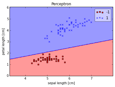
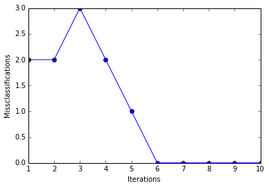
As we can see, the perceptron converges after the 6th iteration and separates the two flower classes perfectly.

Problems with Perceptrons

[back to top]

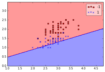
Although the perceptron classified the two Iris flower classes perfectly, convergence is one of the biggest problems of the perceptron. Frank Rosenblatt proofed mathematically that the perceptron learning rule converges if the two classes can be separated by linear hyperplane, but problems arise if the classes cannot be separated perfectly by a linear classifier. To demonstrate this issue, we will use two different classes and features from the Iris dataset.

In [6]:

# versicolor and virginica
y2 = df.iloc[50:150, 4].values
y2 = np.where(y2 == ''Iris-virginica'', -1, 1)

# sepal width and petal width
X2 = df.iloc[50:150, [1,3]].values

ppn = Perceptron(epochs=25, eta=0.01)
ppn.train(X2, y2)

plot_decision_regions(X2, y2, clf=ppn)
plt.show()

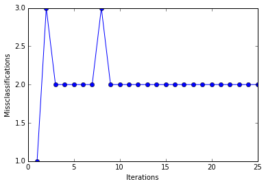
plt.plot(range(1, len(ppn.errors_)+1), ppn.errors_, marker=''o'')
plt.xlabel(''Iterations'')
plt.ylabel(''Misclassifications'')
plt.show()

In [7]:

print(''Total number of misclassifications: %d of 100'' % (y2 != ppn.predict(X2)).sum())

Total number of misclassifications: 43 of 100

Even at a lower training rate, the perceptron failed to find a good decision boundary since one or more samples will always be misclassified in every epoch so that the learning rule never stops updating the weights.

It may seem paradoxical in this context that another shortcoming of the perceptron algorithm is that it stops updating the weights as soon as all samples are classified correctly. Our intuition tells us that a decision boundary with a large margin between the classes (as indicated by the dashed line in the figure below) likely has a better generalization error than the decision boundary of the perceptron. But large-margin classifiers such as Support Vector Machines are a topic for another time.

Adaptive Linear Neurons and the Delta Rule

[back to top]

The perceptron surely was very popular at the time of its discovery, however, it only took a few years until Bernard Widrow and his doctoral student Tedd Hoff proposed the idea of the Adaptive Linear Neuron (adaline) [3].

In contrast to the perceptron rule, the delta rule of the adaline (also known as Widrow-Hoff" rule or Adaline rule) updates the weights based on a linear activation function rather than a unit step function; here, this linear activation function g(z)g(z) is just the identity function of the net input g(wTx)=wTxg(wTx)=wTx. In the next section, we will see why this linear activation is an improvement over the perceptron update and where the name "delta rule" comes from.

Gradient Descent

[back to top]

Being a continuous function, one of the biggest advantages of the linear activation function over the unit step function is that it is differentiable. This property allows us to define a cost function J(w)J(w) that we can minimize in order to update our weights. In the case of the linear activation function, we can define the cost function J(w)J(w) as the sum of squared errors (SSE), which is similar to the cost function that is minimized in ordinary least squares (OLS) linear regression.

J(w)=12∑i(target(i)−output(i))2output(i)∈RJ(w)=12∑i(target(i)−output(i))2output(i)∈R

(The fraction 1212 is just used for convenience to derive the gradient as we will see in the next paragraphs.)

In order to minimize the SSE cost function, we will use gradient descent, a simple yet useful optimization algorithm that is often used in machine learning to find the local minimum of linear systems.

Before we get to the fun part (calculus), let us consider a convex cost function for one single weight. As illustrated in the figure below, we can describe the principle behind gradient descent as "climbing down a hill" until a local or global minimum is reached. At each step, we take a step into the opposite direction of the gradient, and the step size is determined by the value of the learning rate as well as the slope of the gradient.

Now, as promised, onto the fun part -- deriving the Adaline learning rule. As mentioned above, each update is updated by taking a step into the opposite direction of the gradient Δw=−η∇J(w)Δw=−η∇J(w), thus, we have to compute the partial derivative of the cost function for each weight in the weight vector: Δwj=−η∂J∂wjΔwj=−η∂J∂wj.

The partial derivative of the SSE cost function for a particular weight can be calculated as follows:

∂J∂wj=∂∂wj12∑i(t(i)−o(i))2=12∑i∂∂wj(t(i)−o(i))2=12∑i2(t(i)−o(i))∂∂wj(t(i)−o(i))=∑i(t(i)−o(i))∂∂wj(t(i)−∑jwjx(i)j)=∑i(t(i)−o(i))(−x(i)j)(2)(2)∂J∂wj=∂∂wj12∑i(t(i)−o(i))2=12∑i∂∂wj(t(i)−o(i))2=12∑i2(t(i)−o(i))∂∂wj(t(i)−o(i))=∑i(t(i)−o(i))∂∂wj(t(i)−∑jwjxj(i))=∑i(t(i)−o(i))(−xj(i))

(t = target, o = output)

And if we plug the results back into the learning rule, we get

Δwj=−η∂J∂wj=−η∑i(t(i)−o(i))(−x(i)j)=η∑i(t(i)−o(i))x(i)jΔwj=−η∂J∂wj=−η∑i(t(i)−o(i))(−xj(i))=η∑i(t(i)−o(i))xj(i),

Eventually, we can apply a simultaneous weight update similar to the perceptron rule:

w:=w+Δww:=w+Δw.

Although, the learning rule above looks identical to the perceptron rule, we shall note the two main differences:

1. Here, the output "o" is a real number and not a class label as in the perceptron learning rule.
2. The weight update is calculated based on all samples in the training set (instead of updating the weights incrementally after each sample), which is why this approach is also called "batch" gradient descent.

The Gradient Descent Rule in Action

[back to top]

Now, it''s time to implement the gradient descent rule in Python.

In [8]:

import numpy as np

class AdalineGD(object):
    
    def __init__(self, eta=0.01, epochs=50): 
        self.eta = eta
        self.epochs = epochs

    def train(self, X, y):

        self.w_ = np.zeros(1 + X.shape[1])
        self.cost_ = []

        for i in range(self.epochs):
            output = self.net_input(X)
            errors = (y - output)
            self.w_[1:] += self.eta * X.T.dot(errors)
            self.w_[0] += self.eta * errors.sum()
            cost = (errors**2).sum() / 2.0
            self.cost_.append(cost)
        return self

    def net_input(self, X):
        return np.dot(X, self.w_[1:]) + self.w_[0]

    def activation(self, X):
        return self.net_input(X)

    def predict(self, X):
        return np.where(self.activation(X) >= 0.0, 1, -1)

In practice, it often requires some experimentation to find a good learning rate for optimal convergence, thus, we will start by plotting the cost for two different learning rates.

In [9]:

ada = AdalineGD(epochs=10, eta=0.01).train(X, y)
plt.plot(range(1, len(ada.cost_)+1), np.log10(ada.cost_), marker=''o'')
plt.xlabel(''Iterations'')
plt.ylabel(''log(Sum-squared-error)'')
plt.title(''Adaline - Learning rate 0.01'')
plt.show()

ada = AdalineGD(epochs=10, eta=0.0001).train(X, y)
plt.plot(range(1, len(ada.cost_)+1), ada.cost_, marker=''o'')
plt.xlabel(''Iterations'')
plt.ylabel(''Sum-squared-error'')
plt.title(''Adaline - Learning rate 0.0001'')
plt.show()

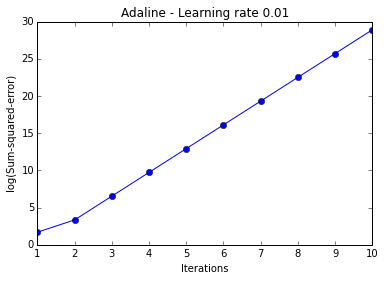
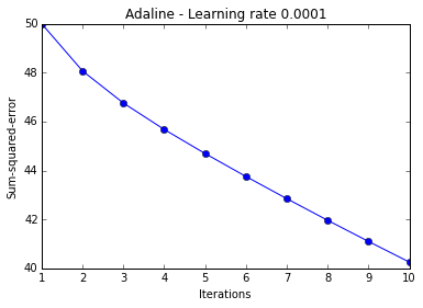
The two plots above nicely emphasize the importance of plotting learning curves by illustrating two most common problems with gradient descent:

1. If the learning rate is too large, gradient descent will overshoot the minima and diverge.
2. If the learning rate is too small, the algorithm will require too many epochs to converge and can become trapped in local minima more easily.

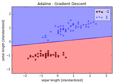
Gradient descent is also a good example why feature scaling is important for many machine learning algorithms. It is not only easier to find an appropriate learning rate if the features are on the same scale, but it also often leads to faster convergence and can prevent the weights from becoming too small (numerical stability).

A common way of feature scaling is standardization

xj,std=xj−μjσjxj,std=xj−μjσj

where μjμj is the sample mean of the feature xjxj and σjσj the standard deviation, respectively. After standardization, the features will have unit variance and are centered around mean zero.

In [10]:

# standardize features
X_std = np.copy(X)
X_std[:,0] = (X[:,0] - X[:,0].mean()) / X[:,0].std()
X_std[:,1] = (X[:,1] - X[:,1].mean()) / X[:,1].std()

In [11]:

%matplotlib inline
import matplotlib.pyplot as plt
from mlxtend.evaluate import plot_decision_regions

ada = AdalineGD(epochs=15, eta=0.01)

ada.train(X_std, y)
plot_decision_regions(X_std, y, clf=ada)
plt.title(''Adaline - Gradient Descent'')
plt.xlabel(''sepal length [standardized]'')
plt.ylabel(''petal length [standardized]'')
plt.show()

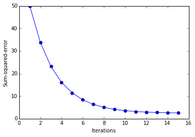
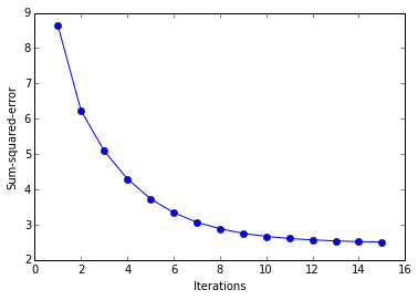
plt.plot(range(1, len( ada.cost_)+1), ada.cost_, marker=''o'')
plt.xlabel(''Iterations'')
plt.ylabel(''Sum-squared-error'')
plt.show()

Online Learning via Stochastic Gradient Descent

[back to top]

The previous section was all about "batch" gradient descent learning. The "batch" updates refers to the fact that the cost function is minimized based on the complete training data set. If we think back to the perceptron rule, we remember that it performed the weight update incrementally after each individual training sample. This approach is also called "online" learning, and in fact, this is also how Adaline was first described by Bernard Widrow et al. [3]

The process of incrementally updating the weights is also called "stochastic" gradient descent since it approximates the minimization of the cost function. Although the stochastic gradient descent approach might sound inferior to gradient descent due its "stochastic" nature and the "approximated" direction (gradient), it can have certain advantages in practice. Often, stochastic gradient descent converges much faster than gradient descent since the updates are applied immediately after each training sample; stochastic gradient descent is computationally more efficient, especially for very large datasets. Another advantage of online learning is that the classifier can be immediately updated as new training data arrives, e.g., in web applications, and old training data can be discarded if storage is an issue. In large-scale machine learning systems, it is also common practice to use so-called "mini-batches", a compromise with smoother convergence than stochastic gradient descent.

In the interests of completeness let us also implement the stochastic gradient descent Adaline and confirm that it converges on the linearly separable iris dataset.

In [14]:

import numpy as np

class AdalineSGD(object):
    
    def __init__(self, eta=0.01, epochs=50):
        self.eta = eta
        self.epochs = epochs

    def train(self, X, y, reinitialize_weights=True):

        if reinitialize_weights:
            self.w_ = np.zeros(1 + X.shape[1])
        self.cost_ = []

        for i in range(self.epochs):
            for xi, target in zip(X, y):
                output = self.net_input(xi)
                error = (target - output)
                self.w_[1:] += self.eta * xi.dot(error)
                self.w_[0] += self.eta * error
            
            cost = ((y - self.activation(X))**2).sum() / 2.0
            self.cost_.append(cost)
        return self

    def net_input(self, X):
        return np.dot(X, self.w_[1:]) + self.w_[0]

    def activation(self, X):
        return self.net_input(X)

    def predict(self, X):
        return np.where(self.activation(X) >= 0.0, 1, -1)

One more advice before we let the adaline learn via stochastic gradient descent is to shuffle the training dataset to iterate over the training samples in random order.

We shall note that the "standard" stochastic gradient descent algorithm uses sampling "with replacement," which means that at each iteration, a training sample is chosen randomly from the entire training set. In contrast, sampling "without replacement," which means that each training sample is evaluated exactly once in every epoch, is not only easier to implement but also shows a better performance in empirical comparisons. A more detailed discussion about this topic can be found in Benjamin Recht and Christopher Re''s paper Beneath the valley of the noncommutative arithmetic-geometric mean inequality: conjectures, case-studies, and consequences [4].

In [15]:

ada = AdalineSGD(epochs=15, eta=0.01)

# shuffle data
np.random.seed(123)
idx = np.random.permutation(len(y))
X_shuffled, y_shuffled =  X_std[idx], y[idx]

# train and adaline and plot decision regions
ada.train(X_shuffled, y_shuffled)
plot_decision_regions(X_shuffled, y_shuffled, clf=ada)
plt.title(''Adaline - Gradient Descent'')
plt.xlabel(''sepal length [standardized]'')
plt.ylabel(''petal length [standardized]'')
plt.show()

plt.plot(range(1, len(ada.cost_)+1), ada.cost_, marker=''o'')
plt.xlabel(''Iterations'')
plt.ylabel(''Sum-squared-error'')
plt.show()

What''s Next?

[back to top]

Although we covered many different topics during this article, we just scratched the surface of artificial neurons.

In later articles, we will take a look at different approaches to dynamically adjust the learning rate, the concepts of "One-vs-All" and "One-vs-One" for multi-class classification, regularization to overcome overfitting by introducing additional information, dealing with nonlinear problems and multilayer neural networks, different activation functions for artificial neurons, and related concepts such as logistic regression and support vector machines.

References

[back to top]

[1] F. Rosenblatt. The perceptron, a perceiving and recognizing automaton Project Para. Cornell Aeronautical Laboratory, 1957.

[2] W. S. McCulloch and W. Pitts. A logical calculus of the ideas immanent in nervous activity. The bulletin of mathematical biophysics, 5(4):115–133, 1943.

[3] B. Widrow et al. Adaptive ”Adaline” neuron using chemical ”memistors”. Number Technical Report 1553-2. Stanford Electron. Labs., Stanford, CA, October 1960.

[4] B. Recht and C. R ́e. Beneath the valley of the noncommutative arithmetic-geometric mean inequality: conjectures, case-studies, and consequences. arXiv preprint arXiv:1202.4184, 2012.

Bilinear CNN与 Randomly Wired Neural Network

最近主要学习了两篇论文以及相关的代码。

1、Bilinear CNN

这篇论文主要是在细粒度分类上应用的，在全连接层之前，在所有的卷积计算完成之后，进行的Bilinear计算，关键的代码如下：

def forward(self, X):
        """Forward pass of the network.

        Args:
            X, torch.autograd.Variable of shape N*3*448*448.

        Returns:
            Score, torch.autograd.Variable of shape N*200.
        """
        N = X.size()[0]
        assert X.size() == (N, 3, 448, 448)
        X = self.features(X)
        assert X.size() == (N, 512, 28, 28)
        X = X.view(N, 512, 28**2)
        X = torch.bmm(X, torch.transpose(X, 1, 2)) / (28**2)  # Bilinear
        assert X.size() == (N, 512, 512)
        X = X.view(N, 512**2)
        X = torch.sqrt(X + 1e-5)
        X = torch.nn.functional.normalize(X)
        X = self.fc(X)
        assert X.size() == (N, 200)
        return X

这个地方和判断卷积核提取的特征的相似度判别，求取的相似矩阵有很大的相似之处。

2、 Randomly Wired Neural Network

将随机图应用到神经网络的构建之中，讲道理，构建的网络其实和DenseNet这种有很大的相似性。具体的过程，寄到笔记本上了。

EfficientNet: Rethinking Model Scaling for Convolutional Neural Networks

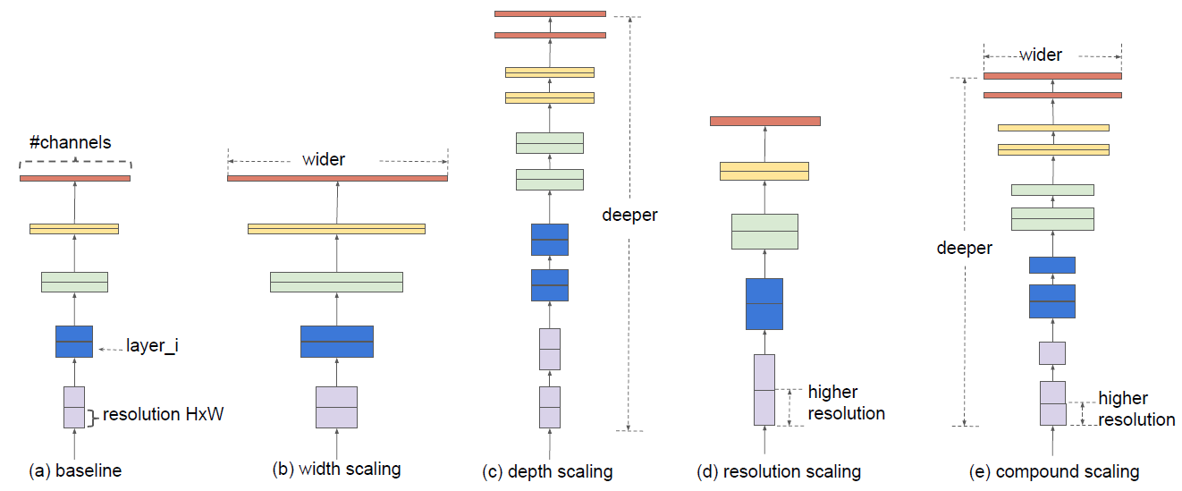
增加模型精度的方法有增加网络的深度，特征图的通道数以及分辨率（如下图a-d所示）。这篇文章研究了模型缩放，发现仔细平衡网络的深度、宽度和分辨率可以获得更好的性能（下图e）。在此基础上，提出了一种新的缩放方法，使用一个简单而高效的复合系数来均匀地标度深度/宽度/分辨率的所有维度，不仅取得了SOTA，而且参数更少，计算复杂度更低。

一个卷积层$i$可以定义为$Y_{i}=\mathcal{F}{i}\left(X{i}\right)$，其中$\mathcal{F}{i}$是操作符，$X_i$是输入张量，形状大小为$\left\langle H{i}, W_{i}, C_{i}\right\rangle$（简单起见，没有引入batchsize），$Y_i$是输出张量，所以一个卷积网络$\mathcal{N}$可以表示为一系列层的组合： $$ \mathcal{N}=\mathcal{F}{k} \odot \ldots \odot \mathcal{F}{2} \odot \mathcal{F}{1}\left(X{1}\right)=\odot_{j=1 \ldots k} \mathcal{F}{j}\left(X{1}\right) $$ 卷积神经网络（如resnet）通常是被分为多个stage的，一个stage的所有层共享相同的结构。因此，上述公式可以变换为： $$ \mathcal{N}=\bigodot_{i=1 \dots s} \mathcal{F}{i}^{L{i}}\left(X_{\left\langle H_{i}, W_{i}, C_{i}\right\rangle}\right) $$ 其中$\mathcal{F}{i}^{L{i}}$表示的是层$F_i$在$stage$ $i$重复了$L_i$次，$\left\langle H_{i}, W_{i}, C_{i}\right\rangle$是第$i$层的输入。根据上面的定义，这篇文章的目标可以抽象成如下公式： $$ \begin{array}{l}{\max {d, w, r} \quad \operatorname{Accuracy}(\mathcal{N}(d, w, r))} \ {\text {s.t.} \quad \mathcal{N}(d, w, r)=\bigoplus{i=1 \ldots s} \hat{\mathcal{F}}{i}^{d \cdot \hat{L}{i}}\left(X_{\left\langle r \cdot \hat{H}{i}, r \cdot \hat{W}{i}, w \cdot \hat{C}_{i}\right\rangle}\right)} \ {\text { Memory }(\mathcal{N}) \leq \text { target-memory }} \ {\text { FLOPS }(\mathcal{N}) \leq \text { target flops }}\end{array} $$ 搜索最优的$d, w, r$，使精确度最高，并且参数量以及运算复杂度不超过目标量。

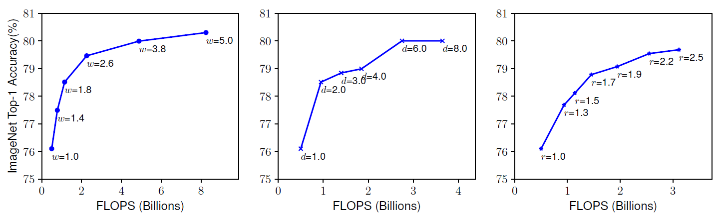
网络深度越深，可以抓取更丰富更复杂的特征，泛化得更好，通道数和分辨率放大，可以抓取更精细化的特征，更好训练。通常是单一的缩放三个中的一个变量，单一扩展网络宽度、深度或分辨率的任何维度都可以提高精度，但是对于更大的模型，精度增益会降低。如下图所示：

文章观察到网络的深度，特征图的通道数以及分辨率三者是互相依赖的，比如，对于更高分辨率的图像而言，我们应该要提高网络深度，这样才会让更大的感受野帮网络在更大图像的更多像素中抓取到相似的特征，同时也应该提高通道数，抓取大图像的更精细的特征。同样，作者也用实验验证了这一点，如下图所示：

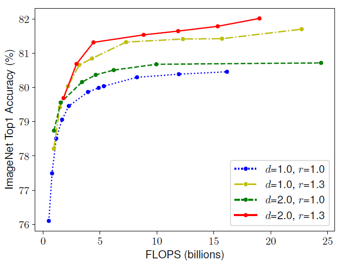
第一个基线网络(d=1.0, r=1.0)有18个卷积层，分辨率为224x224，而最后一个基线(d=2.0, r=1.3)有36层，分辨率为299x299。所以为了追求更高的精度和效率，在ConvNet缩放过程中平衡网络宽度、深度和分辨率的所有维度是至关重要的。

现在来介绍作者提出的方法——复合缩放（compound scaling），该方法使用了一个复合参数$\phi$有原则性地均匀缩放网络深度，宽度以及分辨率。如下公式如示： $$ \begin{aligned} \text { depth: } d &=\alpha^{\phi} \ \text { width: } w &=\beta^{\phi} \ \text { resolution: } r &=\gamma^{\phi} \ \text { s.t. } \alpha & \cdot \beta^{2} \cdot \gamma^{2} \approx 2 \ & \alpha \geq 1, \beta \geq 1, \gamma \geq 1 \end{aligned} $$ $\alpha, \beta, \gamma$皆为常量，可以在很小的栅格中进行搜索，$\phi$可以由用户定义控制资源的缩放因子，加倍网络深度将加倍FLOPS，但加倍网络宽度或分辨率将使FLOPS增加四倍，所以这里的$\beta, \gamma$取的平方，保持三者对于FLOPS的权重是一样的。最终总的FLOPS等于$\left(\alpha \cdot \beta^{2} \cdot \gamma^{2}\right)^{\phi}$，即为$2^\phi$。

复合缩放的方法分为两步：

• 第一步：固定$\phi$为1，这时候的网络（作者命名为EfficientNet-B0）不是很深，对这个网络利用公式2和3对$\alpha, \beta, \gamma$进行搜索，找到最优值。
• 第二步：固定$\alpha, \beta, \gamma$为常数，使用不同$\phi$的公式3放大EfficientNet-B0，依次得到EfficientNet-B1至B7。

看似简单，但效果极佳，各个模型的性能表如下：

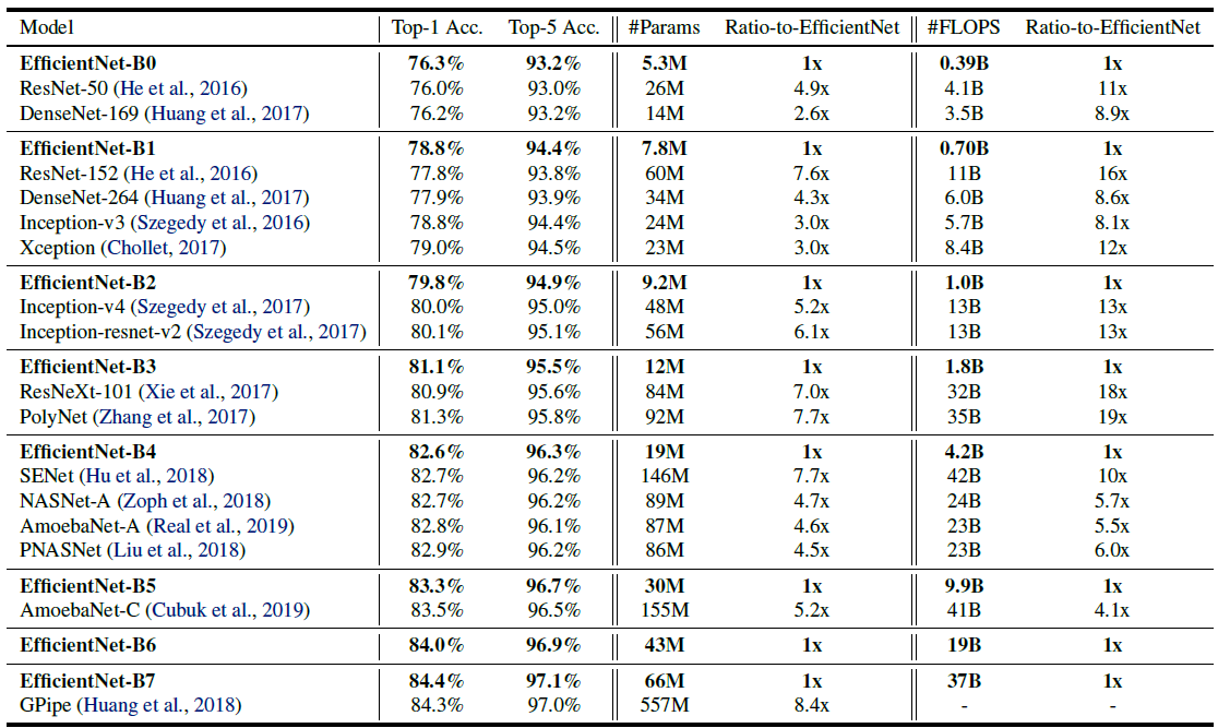
可以看到是又小又快，精度还高，很棒。

GBase8a数据库dblink主要使用场景介绍

8a集群可以通过使用dblink来访问同构集群或异构集群中表的数据，并将读取数据插入到本地表中，这是dblink的主要使用场景。

dblink支持场景如下：

1）支持select语句查询dblink表；

2）支持create…select.. ，select部分使用dblink查询；

3）支持insert..select ..，select部分使用dblink查询；

4）支持多表关联 delete，源部分使用dblink查询；

5）支持存储过程中使用dblink查询；

6）支持prepare语句对dblink查询进行预处理。

dblink不支持场景如下：

1）不支持对dblink表进行DDL操作，如 drop table，alter table等操作；

2）不支持使用dblink表或查询作为update的源关联更新本地表；

3）不支持merge语句using源部分使用dblink查询；

4）不支持function中使用dblink查询。

关于neuralink主要从事什么开发和neuralink公司的问题我们已经讲解完毕，感谢您的阅读，如果还想了解更多关于Artificial Neurons and Single-Layer Neural Networks、Bilinear CNN与 Randomly Wired Neural Network、EfficientNet: Rethinking Model Scaling for Convolutional Neural Networks、GBase8a数据库dblink主要使用场景介绍等相关内容，可以在本站寻找。