写在前面，最近需要在java中调用matplotlib，其他一些画图包都没这个好，毕竟python在科学计算有优势。找到了matplotlib4j，大概看了下github上的https://github.com/sh0nk/matplotlib4j，maven repository：

<dependency>
   <groupId>com.github.sh0nk</groupId>
       <artifactId>matplotlib4j</artifactId>
       <version>0.5.0</version>
</dependency>

简单贴个测试类，更多的用法在test报下有个MainTest.class。

 @Test
    public void testPlot() throws IOException, PythonExecutionException, ClassNotFoundException, NoSuchMethodException, illegalaccessexception, InvocationTargetException, InstantiationException {
        Plot plot = Plot.create(PythonConfig.pythonBinPathConfig("D:\\python3.6\\python.exe"));
        plt.plot()
                .add(Arrays.asList(1.3, 2))
                .label("label")
                .linestyle("--");
        plt.xlabel("xlabel");
        plt.ylabel("ylabel");
        plt.text(0.5, 0.2, "text");
        plt.title("Title!");
        plt.legend();
        plt.show();

    }

下面问题来了，这个对matplotlib的封装不是很全面，源码里也有很多todo，有很多函数简单用用还行，很多重载用不了，比如plt.plot(xdata,ydata)可以，但是无法在其中指定字体plt.plot(xdata,ydata，fontsize=30);

所以想要更全面的用法还得自己动手，几种办法：

1. 大部分还是用matplotlib4j中的，个别的自己需要的但里头没有的函数，实现他的builder接口，重写build方法，返回一个py文件中命令行的字符串形式，然后反射取到PlotImpl中的成员变量registeredBuilders，往后追加命令行，感觉适用于只有极个别命令找不到的情况，挺麻烦的，而且要是传nd.array(…)这种参数还得额外拼字符串。

//拿到plotImpl中用于组装python脚本语句的的registeredBuilders，需要加什么直接添加新的builder就行了
        Field registeredBuildersField = plt.getClass().getDeclaredField("registeredBuilders");
        registeredBuildersField.setAccessible(true);
        List<Builder> registeredBuilders = (List<Builder>) registeredBuildersField.get(plt);

        TicksBuilder ticksBuilder = new TicksBuilder(yList, "yticks", fontSize);
        registeredBuilders.add(ticksBuilder);

2. 这种比较直接，参照matplotlib4j底层，直接写py.exe文件，执行命令行，比较推荐这种，一行一行脚本自己写，数据拼装方便，看起来直观。比如写如下的脚本并执行，搞两组数据，画个散点图

import numpy as np
import matplotlib.pyplot as plt
plt.plot(np.array(自己的x数据), np.array(自己的y数据), 'k.', markersize=4)
plt.xlim(0,6000)
plt.ylim(0,24)
plt.yticks(np.arange(0, 25, 1), fontsize=10)
plt.title("waterfall")
plt.show()

像下面这么写就行了

		//1. 准备自己的数据 不用管
        List<Float> y_secondList_formatByHours = y_secondList.stream().map(second -> (float)second / 3600).collect(Collectors.toList());

        //2.准备命令行list，逐行命令添加
        List<String> scriptLines = new ArrayList<>();
        scriptLines.add("import numpy as np");
        scriptLines.add("import matplotlib.pyplot as plt");
        scriptLines.add("plt.plot("+"np.array("+x_positionList+"),"+"np.array(" +y_secondList_formatByHours+"),\"k.\",label=\"waterfall\",lw=1.0,markersize=4)");
        scriptLines.add("plt.xlim(0,6000)");
        scriptLines.add("plt.ylim(0,24)");
        scriptLines.add("plt.yticks(np.arange(0, 25, 1), fontsize=10)");
        scriptLines.add("plt.title(\"waterfall\")");
        scriptLines.add("plt.show()");
        //3. 调用matplotlib4j 里面的pycommond对象，传入自己电脑的python路径
        pycommand command = new pycommand(PythonConfig.pythonBinPathConfig("D:\\python3.6\\python.exe"));
        //4. 执行，每次执行会生成临时文件 如C:\Users\ADMINI~1\AppData\Local\Temp\1623292234356-0\exec.py，这个带的日志输出能看到，搞定
        command.execute(Joiner.on('\n').join(scriptLines));

linux – 如何从脚本以非阻塞方式执行程序

./a.out -parameters & 
sleep 50 
./b.out -parameters & 
sleep 100 
./c.out &

Matplotlib Superscript format in matplotlib plot legend 上标下标

在绘图的标题、坐标轴的文字中用上标或下标

格式：$正常文字^上标$

import matplotlib.pyplot as plt

fig, ax = plt.subplots()
ax.set(title=r'This is an expression $e^{\sin(\omega\phi)}$',
       xlabel='meters $10^1$', ylabel=r'Hertz $(\frac{1}{s})$')
plt.show()

import matplotlib.pyplot as plt
import numpy as np
from scipy.optimize import curve_fit

x_data = np.linspace(0.05,1,101)
y_data = 1/x_data
noise = np.random.normal(0, 1, y_data.shape)
y_data2 = y_data + noise

def func_power(x, a, b):
    return a*x**b 

popt, pcov= curve_fit(func_power, x_data, y_data2)

plt.figure()
plt.scatter(x_data, y_data2, label = 'data')
plt.plot(x_data, popt[0] * x_data ** popt[1], label = ("$y = {{{}}}x^{{{}}}$").format(round(popt[0],2), round(popt[1],2)))
plt.plot(x_data, x_data**3, label = '$x^3$')
plt.legend()
plt.show()

import matplotlib.pyplot as plt
import numpy as np
from scipy.optimize import curve_fit

x_data = np.linspace(0.05,1,101)
y_data = 1/x_data
noise = np.random.normal(0, 1, y_data.shape)
y_data2 = y_data + noise

def func_power(x, a, b):
    return a*x**b 

popt, pcov= curve_fit(func_power, x_data, y_data2)

plt.figure(figsize=(4, 3))
plt.title('Losses')
plt.ylabel('Loss')
plt.xlabel('Epoch')
plt.scatter(x_data, y_data2, label = 'data')
plt.plot(x_data, popt[0] * x_data ** popt[1], label = ("$y = {{{}}}x^{{{}}}$").format(round(popt[0],2), round(popt[1],2)))
plt.plot(x_data, x_data**3, label = '$x^3$')
plt.legend()
plt.show()

REF

https://stackoverflow.com/questions/53781815/superscript-format-in-matplotlib-plot-legend

 https://stackoverflow.com/questions/21226868/superscript-in-python-plots

Matplotlib Toolkits：三维绘图工具包 matplotlib.mplot3d

http://blog.csdn.net/pipisorry/article/details/40008005

Matplotlib mplot3d 工具包简介

The mplot3d toolkit adds simple 3D plotting capabilities to matplotlib by supplying an axes object that can create a 2D projection of a 3D scene. The resulting graph will have the same look and feel as regular 2D plots.

创建 Axes3D 对象

An Axes3D object is created just like any other axes using the projection=‘3d’ keyword. Create a new matplotlib.figure.Figure and add a new axes to it of type Axes3D:
import matplotlib.pyplot as plt
from mpl_toolkits.mplot3d import Axes3D
fig = plt.figure()
ax = fig.add_subplot(111, projection=’3d’)
New in version 1.0.0: This approach is the preferred method of creating a 3D axes.
Note: Prior to version 1.0.0, the method of creating a 3D axes was di erent. For those using older versions of matplotlib, change ax = fig.add_subplot(111, projection=’3d’) to ax = Axes3D(fig).

要注意的地方

Axes3D 展示三维图形时，其初始视图中 x,y 轴与我们一般看的视图（自己画的时候的视图）是反转的，matlab 也是一样。

Note: 不过这样图形可能会因为旋转而有阴影，也可以通过代码中 XY 轴互换来实现视图中 XY 互换。不知道有没有其它方法，如 matlab 中就有 surf (x,y,z);set (gca,''xdir'',''reverse'',''ydir'',''reverse'') 这样命令来实现这个功能 [关于 matlab 三维图坐标轴原点位置的问题]。

lz 总结绘制三维图形一般流程

创建 Axes3D 对象

fig = plt.figure()
ax = Axes3D(fig)

# 计算坐标极限值
xs = list(itertools.chain.from_iterable([xi[0] for xi in x]))
x_max, x_min = max(xs), min(xs)
ys = list(itertools.chain.from_iterable([xi[1] for xi in x]))
y_max, y_min = max(ys), min(ys)
zs = list(itertools.chain.from_iterable([xi[2] for xi in x]))
z_max, z_min = max(zs), min(zs)
margin = 0.1

再进行绘制，如

plt.scatter(x_new[0], x_new[1], c=''r'', marker=''*'', s=50, label=''new x'')
ax.scatter(xs, ys, zs, c=c, marker=marker, s=50, label=label)
ax.plot_surface(X, Y, Z, rstride=1, cstride=1, label=''Discrimination Interface'')

# 设置图形展示效果
ax.set_xlim(x_min - margin, x_max + margin)
ax.set_ylim(y_min - margin, y_max + margin)
ax.set_zlim(z_min - margin, z_max + margin)
ax.set_xlabel(''x'')
ax.set_ylabel(''y'')
ax.set_zlabel(''z'')
ax.legend(loc=''lower right'')
ax.set_title(''Plot of class0 vs. class1'')
ax.view_init(30, 35)

plt.show()

皮皮 blog

绘制不同三维图形

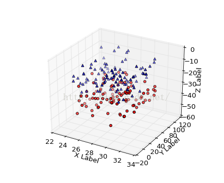
Line plots 线图

Scatter plots 散点图

Axes3D.scatter(xs, ys, zs=0, zdir=u''z'', s=20, c=u''b'', depthshade=True, *args, **kwargs)

Create a scatter plot

Argument	Description
xs, ys	Positions of data points.
zs	Either an array of the same length as xs andys or a single value to place all points inthe same plane. Default is 0.
zdir	Which direction to use as z (‘x’, ‘y’ or ‘z’)when plotting a 2D set.
s	size in points^2. It is a scalar or an array of thesame length as x andy.
c	a color. c can be a single color format string, or asequence of color specifications of lengthN, or asequence ofN numbers to be mapped to colors using thecmap andnorm specified via kwargs (see below). Notethatc should not be a single numeric RGB or RGBAsequence because that is indistinguishable from an arrayof values to be colormapped.c can be a 2-D array inwhich the rows are RGB or RGBA, however.
depthshade	Whether or not to shade the scatter markers to givethe appearance of depth. Default isTrue.

Keyword arguments are passed on to scatter().

Returns a Patch3DCollection

Note: scatter ( x, y, s=20, c=u''b'', marker=u''o'', cmap=None, norm=None, vmin=None, vmax=None, alpha=None, linewidths=None, verts=None, **kwargs )

Wireframe plots 线框图

Surface plots 曲面图

参数

x, y, z: x,y,z 轴对应的数据。注意 z 的数据的 z.shape 是 (len (y), len (x))，不然会报错：ValueError: shape mismatch: objects cannot be broadcast to a single shape

rstride    Array row stride (step size), defaults to 10
cstride    Array column stride (step size), defaults to 10

示例 1：

import numpy as np
import matplotlib.pyplot as plt
from mpl_toolkits.mplot3d import Axes3D

fig = plt.figure()
ax = Axes3D(fig)
X = np.arange(-4, 4, 0.25)
Y = np.arange(-4, 4, 0.25)
X, Y = np.meshgrid(X, Y)
R = np.sqrt(X**2 + Y**2)
Z = np.sin(R)

ax.plot_surface(X, Y, Z, rstride=1, cstride=1, cmap=plt.cm.hot)
ax.contourf(X, Y, Z, zdir=''z'', offset=-2, cmap=plt.cm.hot)
ax.set_zlim(-2,2)

# savefig(''../figures/plot3d_ex.png'',dpi=48)
plt.show()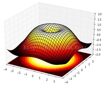

示例 2：

import numpy as np
import matplotlib.pyplot as plt
from mpl_toolkits.mplot3d import Axes3D

fig = plt.figure()
ax = Axes3D(fig)

x = np.arange(0, 200)
y = np.arange(0, 100)
x, y = np.meshgrid(x, y)
z = np.random.randint(0, 200, size=(100, 200))%3
print(z.shape)

# ax.scatter(x, y, z, c=''r'', marker=''.'', s=50, label='''')
ax.plot_surface(x, y, z,label='''')
plt.show()

[surface-plots]

[Matplotlib tutorial - 3D Plots]

Tri-Surface plots 三面图

Contour plots 等高线图

Filled contour plots 填充等高线图

Polygon plots 多边形图

Axes3D.add_collection3d(col, zs=0, zdir=u''z'')

Add a 3D collection object to the plot.

2D collection types are converted to a 3D version bymodifying the object and adding z coordinate information.

Supported are:

• PolyCollection
• LineColleciton
• PatchCollection

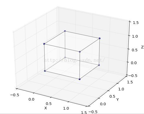
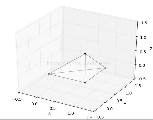
绘制正方体和四面体示例

#!/usr/bin/env python
# -*- coding: utf-8 -*-
"""
__title__ = ''''
__author__ = ''皮''
__mtime__ = ''9/27/2015-027''
__email__ = ''pipisorry@126.com''
"""
import matplotlib.pyplot as plt
from mpl_toolkits.mplot3d.art3d import Poly3DCollection

fig = plt.figure()
ax = fig.gca(projection=''3d'')


# 正文体顶点和面
verts = [(0, 0, 0), (0, 1, 0), (1, 1, 0), (1, 0, 0), (0, 0, 1), (0, 1, 1), (1, 1, 1), (1, 0, 1)]
faces = [[0, 1, 2, 3], [4, 5, 6, 7], [0, 1, 5, 4], [1, 2, 6, 5], [2, 3, 7, 6], [0, 3, 7, 4]]
# 四面体顶点和面
# verts = [(0, 0, 0), (1, 0, 0), (1, 1, 0), (1, 0, 1)]
# faces = [[0, 1, 2], [0, 1, 3], [0, 2, 3], [1, 2, 3]]
# 获得每个面的顶点
poly3d = [[verts[vert_id] for vert_id in face] for face in faces]
# print(poly3d)

# 绘制顶点
x, y, z = zip(*verts)
ax.scatter(x, y, z)
# 绘制多边形面
ax.add_collection3d(Poly3DCollection(poly3d, facecolors=''w'', linewidths=1, alpha=0.3))
# ax.add_collection3d(Line3DCollection(poly3d, colors=''k'', linewidths=0.5, linestyles='':''))

 # 设置图形坐标范围ax.set_xlabel(''X'')ax.set_xlim3d(-0.5, 1.5)ax.set_ylabel(''Y'')ax.set_ylim3d(-0.5, 1.5)ax.set_zlabel(''Z'')ax.set_zlim3d(-0.5, 1.5)plt.show()

绘制结果截图

[Transparency for Poly3DCollection plot in matplotlib]

Bar plots 条形图

2D plots in 3D 三维图中的二维图

Text 文本图

Subplotting 子图

皮皮 blog

matplotlib.mplot3d 绘图实例

matplotlib 绘制 2 维高斯分布

import matplotlib.pyplot as plt
from mpl_toolkits.mplot3d import Axes3D
fig = plt.figure()
ax = Axes3D(fig)
rv = stats.multivariate_normal([0, 0], cov=1)

x, y = np.mgrid[-3:3:.15, -3:3:.15]
ax.plot_surface(x, y, rv.pdf(np.dstack((x, y))), rstride=1, cstride=1)
ax.set_zlim(0, 0.2)

# savefig(''../figures/plot3d_ex.png'',dpi=48)
plt.show()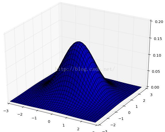

matplotlib 绘制平行 z 轴的平面

（垂直 xy 平面的平面）

方程：0*Z + A [0] X + A [1] Y + A [-1] = 0

X = np.arange(x_min - margin, x_max + margin, 0.05)
Z = np.arange(z_min - margin, z_max + margin, 0.05)
X, Z = np.meshgrid(X, Z)
Y = -1 / A[1] * (A[0] * X + A[-1])
ax.plot_surface(X, Y, Z, rstride=1, cstride=1, label=''Discrimination Interface'')

from:http://blog.csdn.net/pipisorry/article/details/40008005

ref:mplot3d tutorial(inside source code)

mplot3d API

[mplot3d¶]

我们今天的关于使用 Matplotlib 以非阻塞方式绘图和matplotlib fillbetween的分享就到这里，谢谢您的阅读，如果想了解更多关于java版matplotlib，matplotlib4j使用，java中调用matplotlib或者其他python脚本、linux – 如何从脚本以非阻塞方式执行程序、Matplotlib Superscript format in matplotlib plot legend 上标下标、Matplotlib Toolkits：三维绘图工具包 matplotlib.mplot3d的相关信息，可以在本站进行搜索。