如果您对AVisionforMakingDeepLearningSimple感兴趣,那么本文将是一篇不错的选择,我们将为您详在本文中,您将会了解到关于AVisionforMakingDeepLearn
如果您对A Vision for Making Deep Learning Simple感兴趣,那么本文将是一篇不错的选择,我们将为您详在本文中,您将会了解到关于A Vision for Making Deep Learning Simple的详细内容,并且为您提供关于A Gentle Introduction to Transfer Learning for Deep Learning | 迁移学习、Coursera Deep Learning 2 Improving Deep Neural Networks: Hyperparameter tuning, Regularization an...、Creating a simple Pivot table using LINQ and Telerik RadTreeView for Silverlight、Deep Learning (花书) 教材笔记 - Math and Machine Learning Basics (线性代数拾遗)的有价值信息。
本文目录一览:- A Vision for Making Deep Learning Simple
- A Gentle Introduction to Transfer Learning for Deep Learning | 迁移学习
- Coursera Deep Learning 2 Improving Deep Neural Networks: Hyperparameter tuning, Regularization an...
- Creating a simple Pivot table using LINQ and Telerik RadTreeView for Silverlight
- Deep Learning (花书) 教材笔记 - Math and Machine Learning Basics (线性代数拾遗)

A Vision for Making Deep Learning Simple
A Vision for Making Deep Learning Simple
When MapReduce was introduced 15 years ago, it showed the world a glimpse into the future. For the first time, engineers at Silicon Valley tech companies could analyze the entire Internet. MapReduce, however, provided low-level APIs that were incredibly difficult to use, and as a result, this “superpower” was a luxury — only a small fraction of highly sophisticated engineers with lots of resources could afford to use it.
Today, deep learning has reached its “MapReduce” point: it has demonstrated its potential; it is the “superpower” of Artificial Intelligence. Its accomplishments were unthinkable a few years ago: self-driving cars and AlphaGo would have been considered miracles.
Yet leveraging the superpower of deep learning today is as challenging as big data was yesterday: deep learning frameworks have steep learning curves because of low-level APIs; scaling out over distributed hardware requires significant manual work; and even with the combination of time and resources, achieving success requires tedious fiddling and experimenting with parameters. Deep learning is often referred to as “black magic.”
Seven years ago, a group of us started the Spark project with the singular goal to “democratize” the “superpower” of big data, by offering high-level APIs and a unified engine to do machine learning, ETL, streaming and interactive SQL. Today, Apache Spark makes big data accessible to everyone from software engineers to SQL analysts.
Continuing with that vision of democratization, we are excited to announce Deep Learning Pipelines, a new open-source library aimed at enabling everyone to easily integrate scalable deep learning into their workflows, from machine learning practitioners to business analysts.
Deep Learning Pipelines builds on Apache Spark’s ML Pipelines for training, and with Spark DataFrames and SQL for deploying models. It includes high-level APIs for common aspects of deep learning so they can be done efficiently in a few lines of code:
- Image loading
- Applying pre-trained models as transformers in a Spark ML pipeline
- Transfer learning
- Distributed hyperparameter tuning
- Deploying models in DataFrames and SQL
In the rest of the post, we describe each of these features in detail with examples. To try out these and further examples on Databricks, check out the notebook Deep Learning Pipelines on Databricks.
Image Loading
The first step to applying deep learning on images is the ability to load the images. Deep Learning Pipelines includes utility functions that can load millions of images into a DataFrame and decode them automatically in a distributed fashion, allowing manipulation at scale.
df = imageIO.readImages("/data/myimages")We are also working on adding support for more data types, such as text and time series.
Applying Pre-trained Models for Scalable Prediction
Deep Learning Pipelines supports running pre-trained models in a distributed manner with Spark, available in both batch and streaming data processing. It houses some of the most popular models, enabling users to start using deep learning without the costly step of training a model. For example, the following code creates a Spark prediction pipeline using InceptionV3, a state-of-the-art convolutional neural network (CNN) model for image classification, and predicts what objects are in the images that we just loaded. This prediction, of course, is done in parallel with all the benefits that come with Spark:
from sparkdl import readImages, DeepImagePredictor
predictor = DeepImagePredictor(inputCol="image", outputCol="predicted_labels", modelName="InceptionV3")
predictions_df = predictor.transform(df)
In addition to using the built-in models, users can plug in Keras models and TensorFlow Graphs in a Spark prediction pipeline. This turns any single-node models on single-node tools into one that can be applied in a distributed fashion, on a large amount of data.
On Databricks’ Unified Analytics Platform, if you choose a GPU-based cluster, the computation intensive parts will automatically run on GPUs for best efficiency.
Transfer Learning
Pre-trained models are extremely useful when they are suitable for the task at hand, but they are often not optimized for the specific dataset users are tackling. As an example, InceptionV3 is a model optimized for image classification on a broad set of 1000 categories, but our domain might be dog breed classification. A commonly used technique in deep learning is transfer learning, which adapts a model trained for a similar task to the task at hand. Compared with training a new model from ground-up, transfer learning requires substantially less data and resources. This is why transfer learning has become the go-to method in many real world use cases, such as cancer detection.
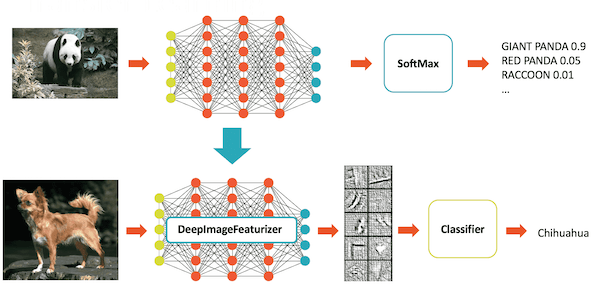
Deep Learning Pipelines enables fast transfer learning with the concept of a Featurizer. The following example combines the InceptionV3 model and logistic regression in Spark to adapt InceptionV3 to our specific domain. The DeepImageFeaturizer automatically peels off the last layer of a pre-trained neural network and uses the output from all the previous layers as features for the logistic regression algorithm. Since logistic regression is a simple and fast algorithm, this transfer learning training can converge quickly using far fewer images than are typically required to train a deep learning model from ground-up.
from sparkdl import DeepImageFeaturizer
from pyspark.ml.classification import LogisticRegression

featurizer = DeepImageFeaturizer(modelName="InceptionV3")
lr = LogisticRegression()
p = Pipeline(stages=[featurizer, lr])

# train_images_df = ... # load a dataset of images and labels
model = p.fit(train_images_df)
Distributed Hyperparameter Tuning
Getting the best results in deep learning requires experimenting with different values for training parameters, an important step called hyperparameter tuning. Since Deep Learning Pipelines enables exposing deep learning training as a step in Spark’s machine learning pipelines, users can rely on the hyperparameter tuning infrastructure already built into Spark.

The following code plugs in a Keras Estimator and performs hyperparameter tuning using grid search with cross validation:
myEstimator = KerasImageFileEstimator(inputCol=''input'',
                                      outputCol=''output'',
                                      modelFile=''/my_models/model.h5'',
                                      imageLoader=_loadProcessKeras)

kerasParams1 = {''batch_size'':10, epochs:10}
kerasParams2 = {''batch_size'':5, epochs:20}

myParamMaps =
  ParamGridBuilder() \
    .addGrid(myEstimator.kerasParams, [kerasParams1, kerasParams2]) \
    .build()

cv = CrossValidator(myEstimator, myEvaluator, myParamMaps)
cvModel = cv.fit()
kerasTransformer = cvModel.bestModel  # of type KerasTransformer
Deploying Models in SQL
Once a data scientist builds the desired model, Deep Learning Pipelines makes it simple to expose it as a function in SQL, so anyone in their organization can use it – data engineers, data scientists, business analysts, anybody.
sparkdl.registerKerasUDF("img_classify", "/mymodels/dogmodel.h5")Next, any user in the organization can apply prediction in SQL:
SELECT image, img_classify(image) label FROM images
WHERE contains(label, “Chihuahua”)
Similar functionality is also available in the DataFrame programmatic API across all supported languages (Python, Scala, Java, R). Similar to scalable prediction, this feature works in both batch and structured streaming.
Conclusion
In this blog post, we introduced Deep Learning Pipelines, a new library that makes deep learning drastically easier to use and scale. While this is just the beginning, we believe Deep Learning Pipelines has the potential to accomplish what Spark did to big data: make the deep learning “superpower” approachable for everybody.
Future posts in the series will cover the various tools in the library in more detail: image manipulation at scale, transfer learning, prediction at scale, and making deep learning available in SQL.
To learn more about the library, check out the Databricks notebook as well as the github repository. We encourage you to give us feedback. Or even better, be a contributor and help bring the power of scalable deep learning to everyone.

A Gentle Introduction to Transfer Learning for Deep Learning | 迁移学习
by Jason Brownlee on December 20, 2017 in Better Deep Learning
Transfer learning is a machine learning method where a model developed for a task is reused as the starting point for a model on a second task.
It is a popular approach in deep learning where pre-trained models are used as the starting point on computer vision and natural language processing tasks given the vast compute and time resources required to develop neural network models on these problems and from the huge jumps in skill that they provide on related problems.
In this post, you will discover how you can use transfer learning to speed up training and improve the performance of your deep learning model.
After reading this post, you will know:
- What transfer learning is and how to use it.
- Common examples of transfer learning in deep learning.
- When to use transfer learning on your own predictive modeling problems.
Let’s get started.
What is Transfer Learning?
Transfer learning is a machine learning technique where a model trained on one task is re-purposed on a second related task.
Transfer learning and domain adaptation refer to the situation where what has been learned in one setting … is exploited to improve generalization in another setting
— Page 526, Deep Learning, 2016.
Transfer learning is an optimization that allows rapid progress or improved performance when modeling the second task.
Transfer learning is the improvement of learning in a new task through the transfer of knowledge from a related task that has already been learned.
— Chapter 11: Transfer Learning, Handbook of Research on Machine Learning Applications, 2009.
Transfer learning is related to problems such as multi-task learning and concept drift and is not exclusively an area of study for deep learning.
Nevertheless, transfer learning is popular in deep learning given the enormous resources required to train deep learning models or the large and challenging datasets on which deep learning models are trained.
Transfer learning only works in deep learning if the model features learned from the first task are general.
In transfer learning, we first train a base network on a base dataset and task, and then we repurpose the learned features, or transfer them, to a second target network to be trained on a target dataset and task. This process will tend to work if the features are general, meaning suitable to both base and target tasks, instead of specific to the base task.
— How transferable are features in deep neural networks?
This form of transfer learning used in deep learning is called inductive transfer. This is where the scope of possible models (model bias) is narrowed in a beneficial way by using a model fit on a different but related task.

Depiction of Inductive Transfer
Taken from “Transfer Learning”
How to Use Transfer Learning?
You can use transfer learning on your own predictive modeling problems.
Two common approaches are as follows:
- Develop Model Approach
- Pre-trained Model Approach
Develop Model Approach
- Select Source Task. You must select a related predictive modeling problem with an abundance of data where there is some relationship in the input data, output data, and/or concepts learned during the mapping from input to output data.
- Develop Source Model. Next, you must develop a skillful model for this first task. The model must be better than a naive model to ensure that some feature learning has been performed.
- Reuse Model. The model fit on the source task can then be used as the starting point for a model on the second task of interest. This may involve using all or parts of the model, depending on the modeling technique used.
- Tune Model. Optionally, the model may need to be adapted or refined on the input-output pair data available for the task of interest.
Pre-trained Model Approach
- Select Source Model. A pre-trained source model is chosen from available models. Many research institutions release models on large and challenging datasets that may be included in the pool of candidate models from which to choose from.
- Reuse Model. The model pre-trained model can then be used as the starting point for a model on the second task of interest. This may involve using all or parts of the model, depending on the modeling technique used.
- Tune Model. Optionally, the model may need to be adapted or refined on the input-output pair data available for the task of interest.
This second type of transfer learning is common in the field of deep learning.
Examples of Transfer Learning with Deep Learning
Let’s make this concrete with two common examples of transfer learning with deep learning models.
Transfer Learning with Image Data
It is common to perform transfer learning with predictive modeling problems that use image data as input.
This may be a prediction task that takes photographs or video data as input.
For these types of problems, it is common to use a deep learning model pre-trained for a large and challenging image classification task such as the ImageNet 1000-class photograph classification competition.
The research organizations that develop models for this competition and do well often release their final model under a permissive license for reuse. These models can take days or weeks to train on modern hardware.
These models can be downloaded and incorporated directly into new models that expect image data as input.
Three examples of models of this type include:
- Oxford VGG Model
- Google Inception Model
- Microsoft ResNet Model
For more examples, see the Caffe Model Zoo where more pre-trained models are shared.
This approach is effective because the images were trained on a large corpus of photographs and require the model to make predictions on a relatively large number of classes, in turn, requiring that the model efficiently learn to extract features from photographs in order to perform well on the problem.
In their Stanford course on Convolutional Neural Networks for Visual Recognition, the authors caution to carefully choose how much of the pre-trained model to use in your new model.
[Convolutional Neural Networks] features are more generic in early layers and more original-dataset-specific in later layers
— Transfer Learning, CS231n Convolutional Neural Networks for Visual Recognition
Transfer Learning with Language Data
It is common to perform transfer learning with natural language processing problems that use text as input or output.
For these types of problems, a word embedding is used that is a mapping of words to a high-dimensional continuous vector space where different words with a similar meaning have a similar vector representation.
Efficient algorithms exist to learn these distributed word representations and it is common for research organizations to release pre-trained models trained on very large corpa of text documents under a permissive license.
Two examples of models of this type include:
- Google’s word2vec Model
- Stanford’s GloVe Model
These distributed word representation models can be downloaded and incorporated into deep learning language models in either the interpretation of words as input or the generation of words as output from the model.
In his book on Deep Learning for Natural Language Processing, Yoav Goldberg cautions:
… one can download pre-trained word vectors that were trained on very large quantities of text […] differences in training regimes and underlying corpora have a strong influence on the resulting representations, and that the available pre-trained representations may not be the best choice for [your] particular use case.
— Page 135, Neural Network Methods in Natural Language Processing, 2017.
When to Use Transfer Learning?
Transfer learning is an optimization, a shortcut to saving time or getting better performance.
In general, it is not obvious that there will be a benefit to using transfer learning in the domain until after the model has been developed and evaluated.
Lisa Torrey and Jude Shavlik in their chapter on transfer learning describe three possible benefits to look for when using transfer learning:
- Higher start. The initial skill (before refining the model) on the source model is higher than it otherwise would be.
- Higher slope. The rate of improvement of skill during training of the source model is steeper than it otherwise would be.
- Higher asymptote. The converged skill of the trained model is better than it otherwise would be.

Three ways in which transfer might improve learning.
Taken from “Transfer Learning”.
Ideally, you would see all three benefits from a successful application of transfer learning.
It is an approach to try if you can identify a related task with abundant data and you have the resources to develop a model for that task and reuse it on your own problem, or there is a pre-trained model available that you can use as a starting point for your own model.
On some problems where you may not have very much data, transfer learning can enable you to develop skillful models that you simply could not develop in the absence of transfer learning.
The choice of source data or source model is an open problem and may require domain expertise and/or intuition developed via experience.
Further Reading
This section provides more resources on the topic if you are looking to go deeper.
Books
- Deep Learning, 2016.
- Neural Network Methods in Natural Language Processing, 2017.
Papers
- A survey on transfer learning, 2010.
- Chapter 11: Transfer Learning, Handbook of Research on Machine Learning Applications, 2009.
- How transferable are features in deep neural networks?
Pre-trained Models
- Oxford VGG Model
- Google Inception Model
- Microsoft ResNet Model
- Google’s word2vec Model
- Stanford’s GloVe Model
- Caffe Model Zoo
Articles
- Transfer learning on Wikipedia
- Transfer Learning – Machine Learning’s Next Frontier, 2017.
- Transfer Learning, CS231n Convolutional Neural Networks for Visual Recognition
- How does transfer learning work? on Quora
Summary
In this post, you discovered how you can use transfer learning to speed up training and improve the performance of your deep learning model.
Specifically, you learned:
- What transfer learning is and how it is used in deep learning.
- When to use transfer learning.
- Examples of transfer learning used on computer vision and natural language processing tasks.

Coursera Deep Learning 2 Improving Deep Neural Networks: Hyperparameter tuning, Regularization an...
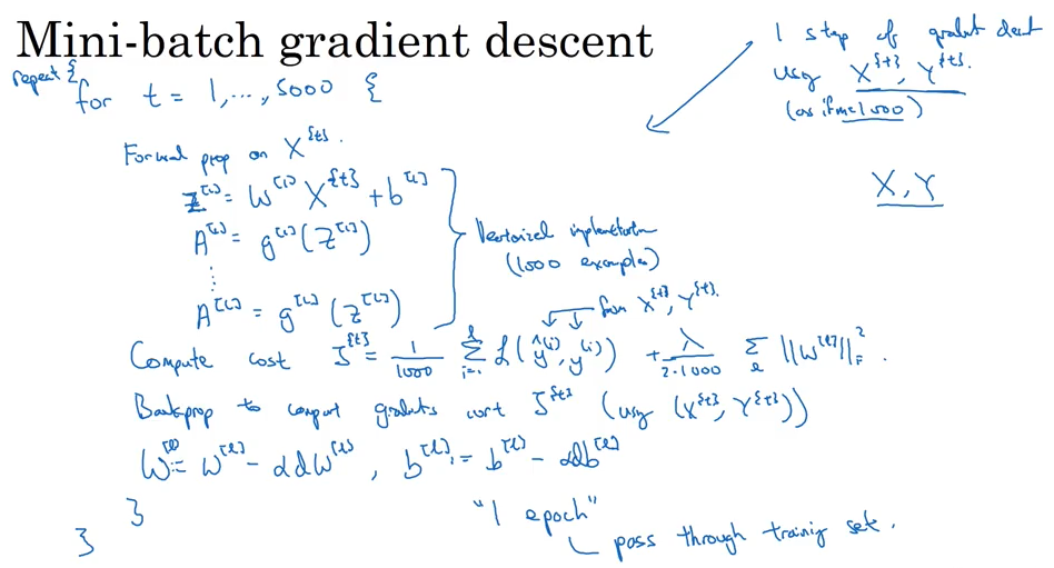
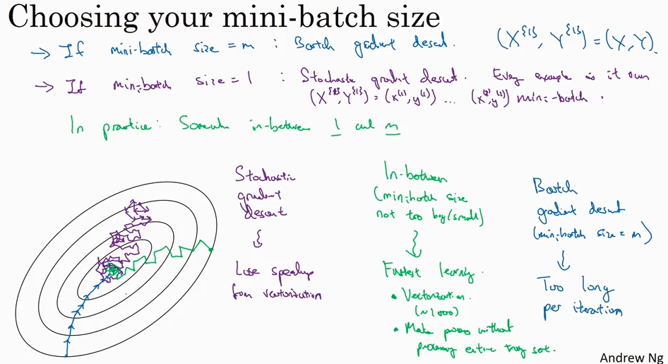
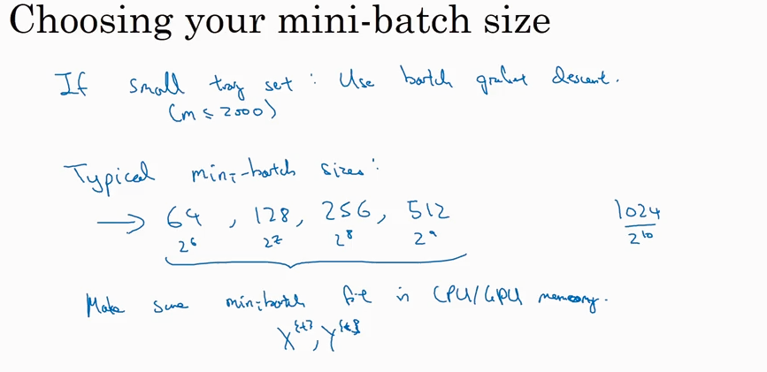
Gradient descent
Batch Gradient Decent, Mini-batch gradient descent, Stochastic gradient descent
还有很多比gradient decent 更优化的算法,在了解这些算法前,需要先理解 Exponentially weighted averages 这个概念
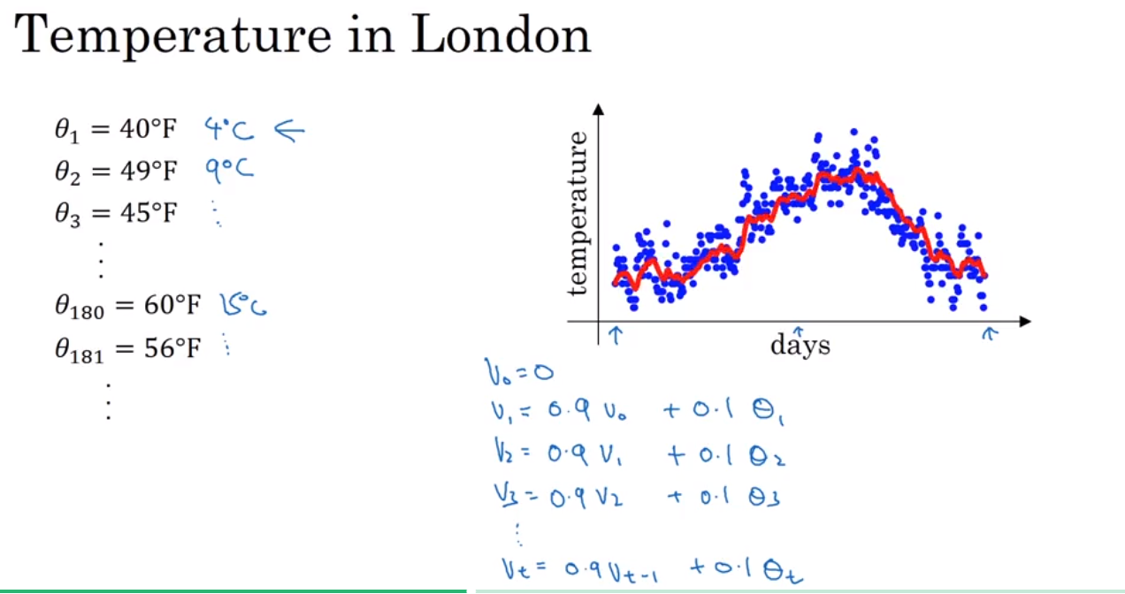

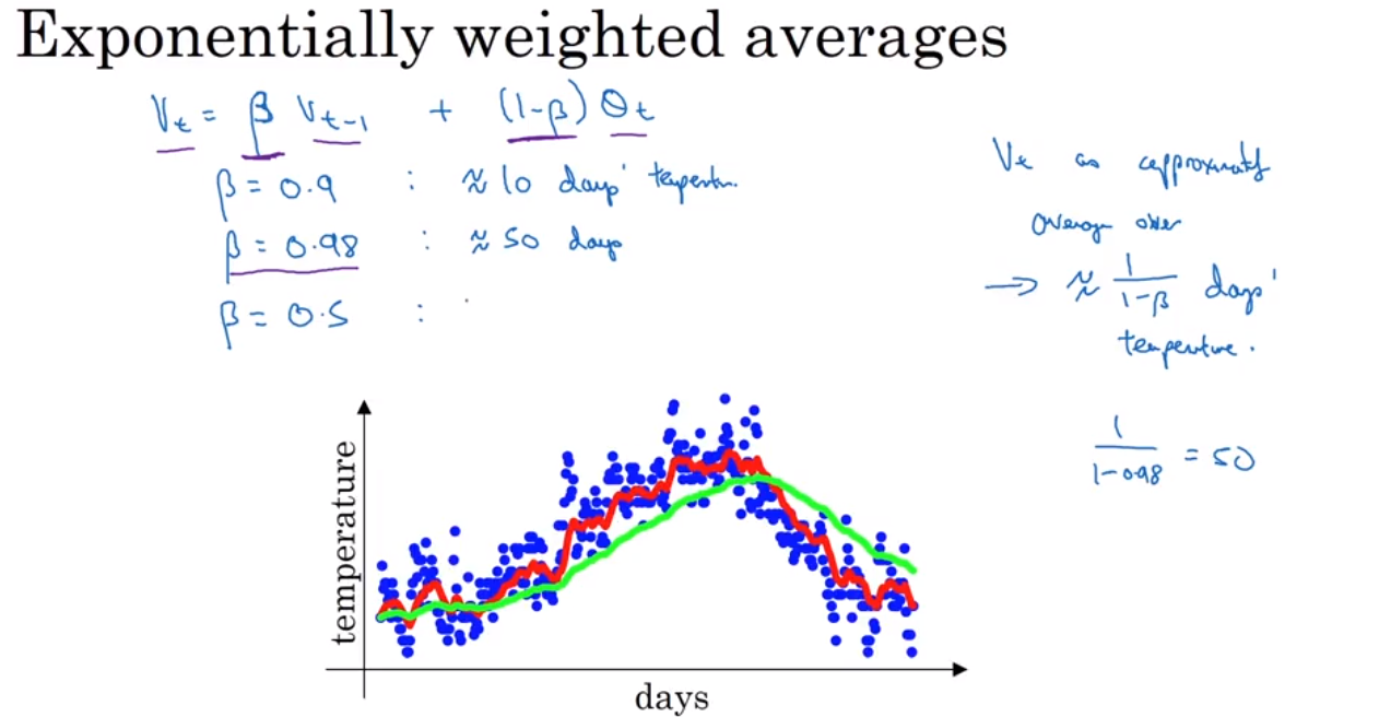
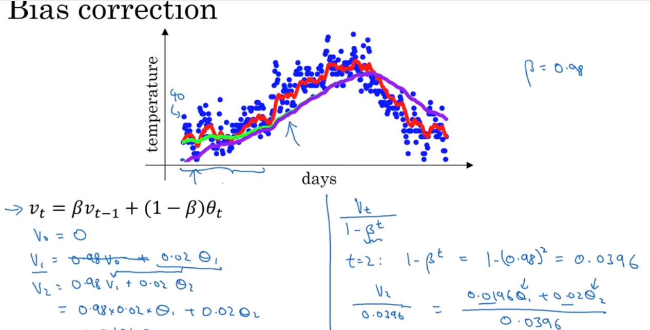
Exponentially weighted average 是一种计算平均值的方法,非常省storage 和 memory, 但是不是很精确。 然后引出一个bias correction 的概念,就是为了能使得 Exponentially weighted average 更加精确.
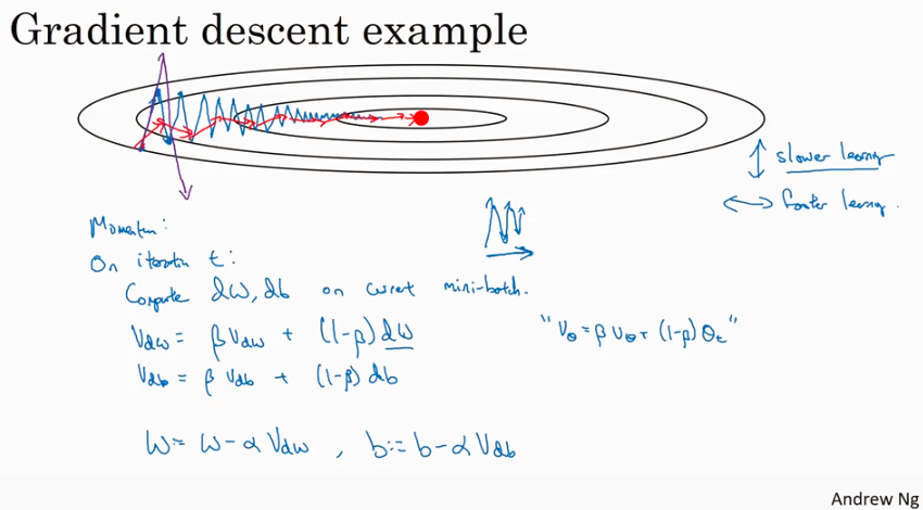
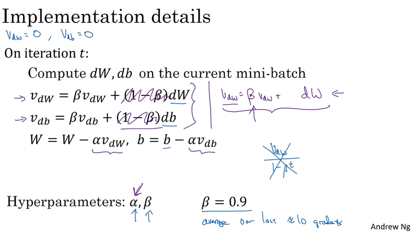
momentum (or called Gradient descent with momentum)
传统的Gradient descent 算法有如下图所示的问题 - 每次迭代都会来回跳动,不直接指向optimum, 在没有做feature scaling 的时候尤其明显。所以引出一个修正的算法 - Gradient descent with momentum.
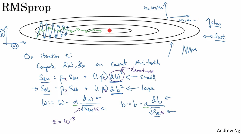
RMSprop
目的和上面讲到的Momentum是一样的,就是使得每次迭代都尽量指向optimum而不是来回跳动. 算法实现如下. RMSprop带来的好处是迭代更快,和可以选用更大的learning rate.
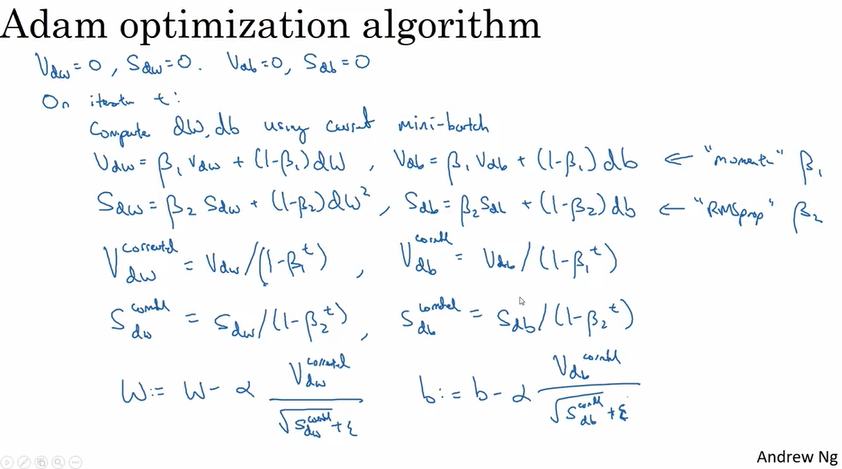
Adam optimation algorithm:
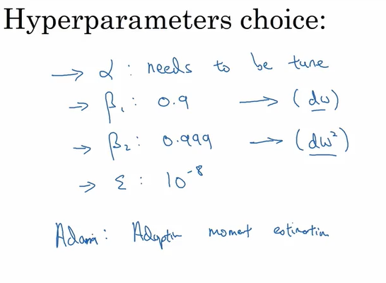
结合了Momentum 和 RMSprop 两种算法. Adam stands for Adaptive mement estimation.
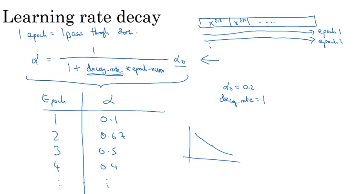
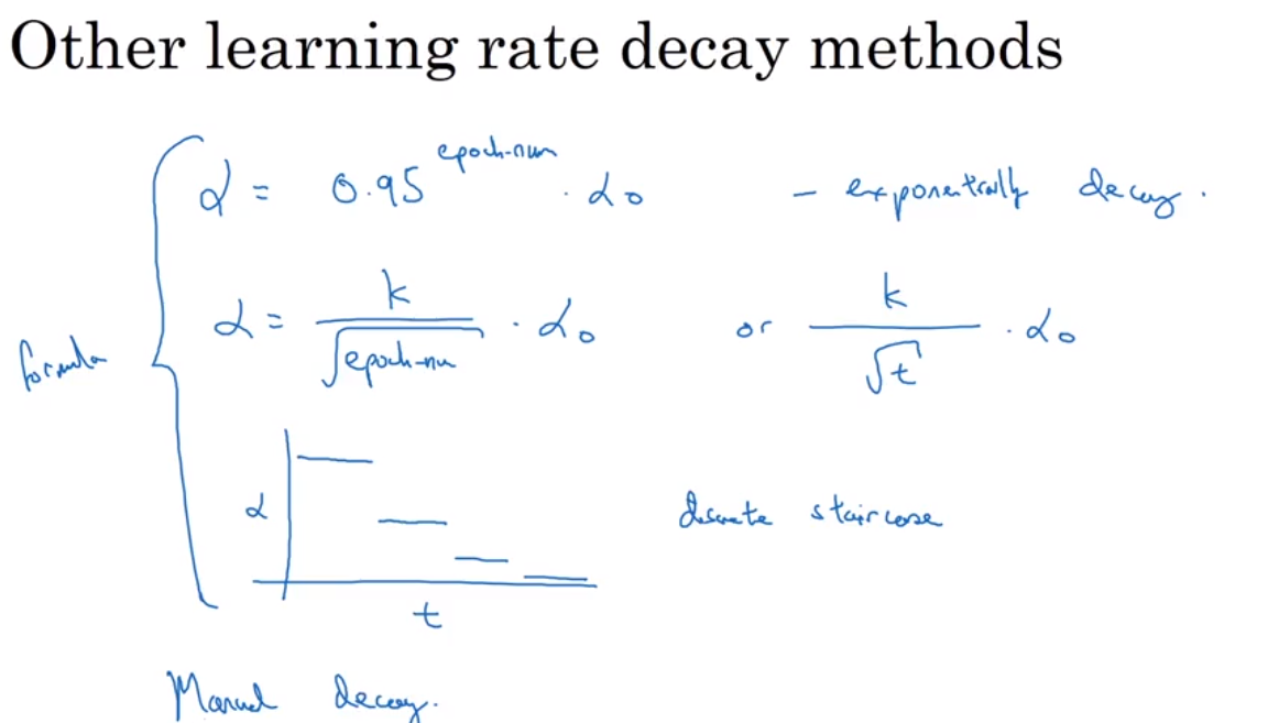
Learning rate decay
why? to reduce the oscillation near the central point.
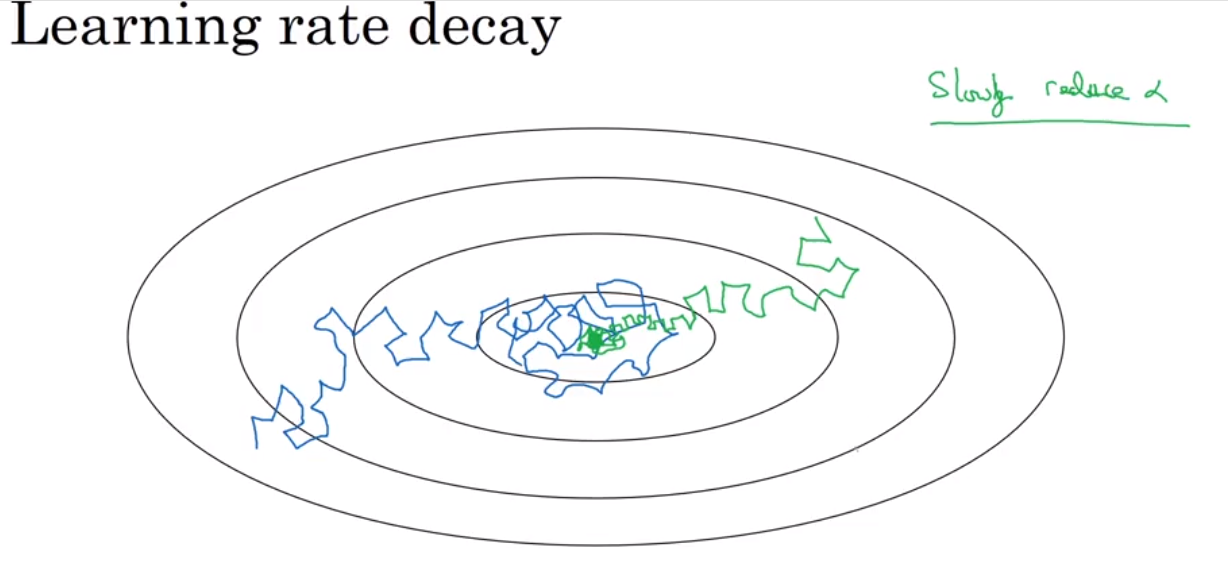
有哪些实现方式呢?
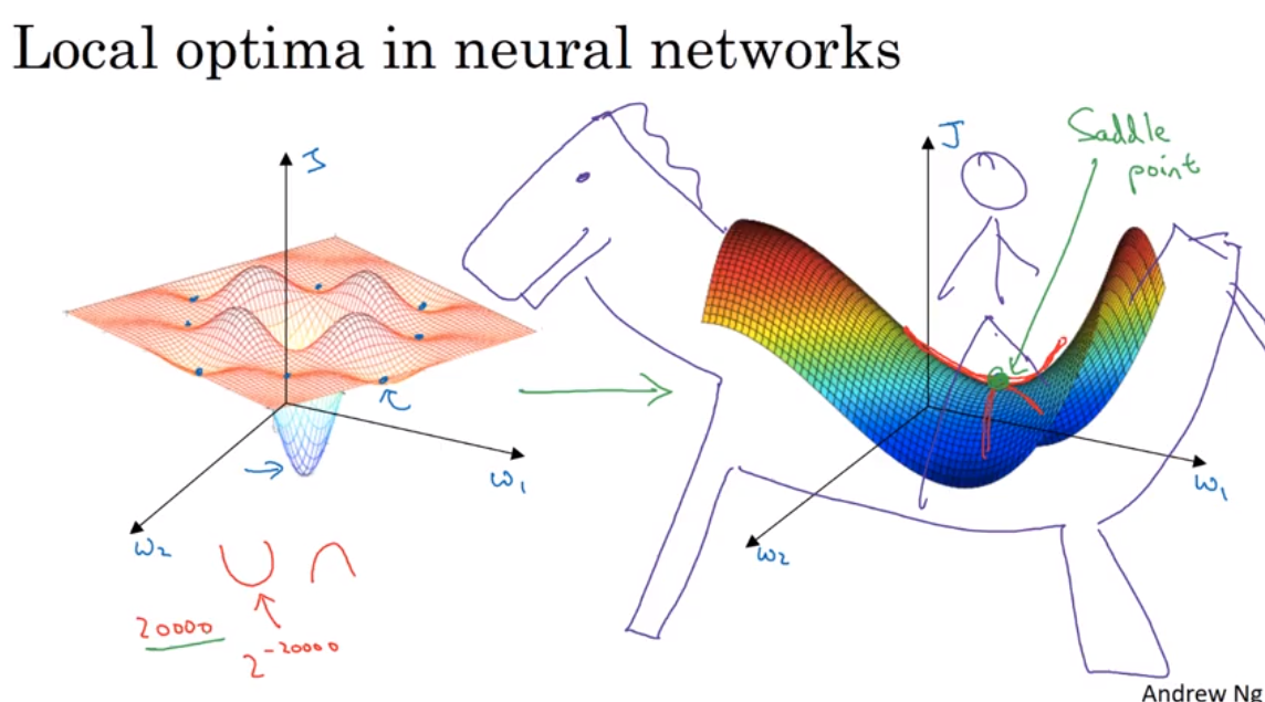
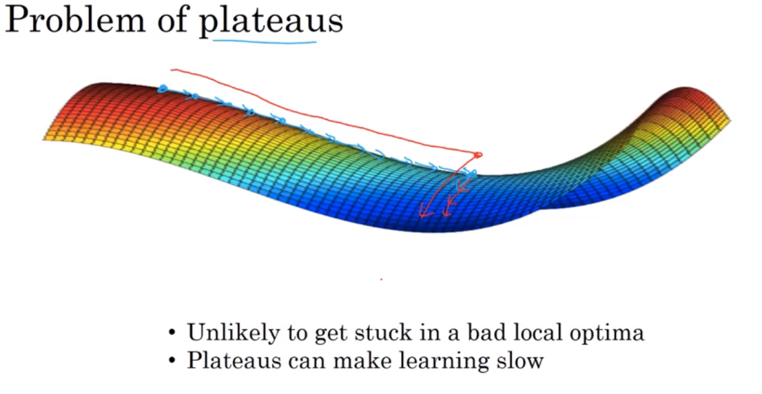
Local optima and saddle point
在大型神经网络里,saddle point 可能比local optima更常见.
Ref:
Coursera, Deep leaning, Andrew Ng

Creating a simple Pivot table using LINQ and Telerik RadTreeView for Silverlight
This article is compatible with the latest version of Silverlight.
What is a Pivot table/grid? According to Wikipedia it is a data summarization tool found in spreadsheet applications. Still when I was a child I learned that people understand the best when they see an example.
Consider you have a table that contains the nutrition of given food,say a pizza:
| Group | Name | Quantity |
| Carbohydrates | Total carbohydrates | 27.3 |
| Carbohydrates | Total disaccharides | 5.7 |
| Carbohydrates | Total polysaccharides | 21.6 |
| minerals | Calcium | 147 |
| minerals | Phosphorus | 150 |
| minerals | Potassium | 201 |
| minerals | copper | 0.13 |
| minerals | Magnesium | 19 |
| minerals | sodium | 582 |
| minerals | Selenium | 4 |
| minerals | Total iron | 0.7 |
| minerals | Zinc | 1.07 |
| Vitamins | Beta-carotene | 173.8 |
| Vitamins | Nicotinic | 1.5 |
| Vitamins | Total vitamin B6 | 0.127 |
| Vitamins | Total vitamin D | 0.3 |
| Vitamins | Total vitamin E | 2.1 |
| Vitamins | Vitamin B1 | 0.1 |
| Vitamins | Vitamin B12 | 0.59 |
| Vitamins | Vitamin B2 | 0.16 |
| Vitamins | Vitamin C | 10 |
In the data above you see that every nutrition is contained in a specific Group - 3 groups and 21 nutrition in total. To display the nutrition in a more meaningful way in most cases you need to group the nutrition (rows in the general case) by their Group attribute and display them in columns instead of in rows. Now we are closer to what we call a Pivot table - group and turn rows into columns.
So the above table displayed in a Pivot would look like that:
| Carbohydrates | minerals | Vitamins | |||
| Total carbohydrates | 27.3 | Calcium | 147 | Beta-carotene | 173.8 |
| Total disaccharides | 5.7 | Phosphorus | 150 | Nicotinic | 1.5 |
| Total polysaccharides | 21.6 | Potassium | 201 | Total vitamin B6 | 0.127 |
| copper | 0.13 | Total vitamin D | 0.3 | ||
| Magnesium | 19 | Total vitamin E | 2.1 | ||
| sodium | 582 | Vitamin B1 | 0.1 | ||
| Selenium | 4 | Vitamin B12 | 0.59 | ||
| Total iron | 0.7 | Vitamin B2 | 0.16 | ||
| Zinc | 1.07 | Vitamin C | 10 |
I searched for a 3rd party control that can help me achieve this goal out of the Box,but I Couldn't find one. Looking for a way to do it I finally made it work with the help of LINQ - for grouping and the Telerik RadTreeView for Silverlight - for displaying.
Loading the data with LINQ
First,consider we have the initial table of nutrition exported to XML. The output look like that:
<?xmlversion="1.0"encoding="utf-8"?><Nutritions> <NutritionGroup="Carbohydrates"Name="Total carbohydrates"Quantity="27.3"></Nutrition> <NutritionGroup="Carbohydrates"Name="Total disaccharides"Quantity="5.7"></Nutrition> <NutritionGroup="Carbohydrates"Name="Total polysaccharides"Quantity="21.6"></Nutrition> <NutritionGroup="minerals"Name="Calcium"Quantity="147"></Nutrition> <NutritionGroup="minerals"Name="Phosphorus "Quantity="150"></Nutrition>
Create a business object Nutrition that will be used later when loading the XML with LINQ.
publicclassNutrition{ publicstringGroup {get;set; } publicstringName {get;set; } publicstringQuantity {get;set; }}
and NutritionGroup:
public class NutritionGroup
{
public string NutritionGroupHeader { get; set; }
public Collection<Nutrition> Nutritions { get; set; }
}
Now,it's time to load the XML document with LINQ. Martin Mihaylov published a great article on using LINQ to XML in Silverlight so if you are not familiar you'd better go read it first.
List data = ( from nutritioninnutritionsDoc.Descendants("Nutrition") selectnewNutrition { Group = nutrition.Attribute("Group").Value, Name = nutrition.Attribute("Name").Value, Quantity = nutrition.Attribute("Quantity").Value } ).ToList();
Grouping the data with LINQ and building the tree
Ok,this is the core of this article. The ability to group is a great feature in LINQ. It really does simplify the code to minimum.
We need to group by the Group attribute.
IEnumerable<string,Nutrition>> query = data.GroupBy( nutrition => nutrition.Group );
Now,each nutrition group should be a root node in the tree and each nutrition in this group should be added to the nutritions in the corresponding root. When the ItemSource property is set to the collection of nutrition groups,the RadTreeView will be populated with the corresponding data:
Collection<NutritionGroup> nutritions =newCollection<NutritionGroup>();foreach( IGrouping<string,Nutrition> nutritionGroupinquery ){ NutritionGroup group =newNutritionGroup() { NutritionGroupHeader = nutritionGroup.Key, }; group.Nutritions =newCollection<Nutrition>(); foreach( Nutrition nutritioninnutritionGroup ) { group.Nutritions.Add( nutrition ); } nutritions.Add( group );}nutritionTree.ItemsSource = nutritions;
Ok,we are almost over. Let's take a look at the NutritionGroupTemplate and NutritionTemplate that we will use. First,we will need the following schema:
xmlns:telerik="http://schemas.telerik.com/2008/xaml/presentation"
Having that,follows both the templates:
NutritionGroupTemplate
<telerik:HierarchicalDataTemplatex:Key="NutritionGroupTemplate" ItemsSource="{Binding Nutritions}"ItemTemplate="{StaticResource NutritionTemplate}"> <BorderBorderThickness="1"BorderBrush="#ececec"CornerRadius="4"> <BorderBorderThickness="1"BorderBrush="White"Padding="1"CornerRadius="4"> <Border.Background> <LinearGradientBrushEndPoint="0.5,1"StartPoint="0.5,0"> <GradientStopColor="#f8f8f8"/> <GradientStopColor="#ececec"Offset="1"/> </LinearGradientBrush> </Border.Background> <TextBlockText="{Binding NutritionGroupHeader}"FontWeight="Bold"/> </Border> </Border></telerik:HierarchicalDataTemplate>
NutritionTemplate
<telerik:HierarchicalDataTemplatex:Key="NutritionTemplate"> <StackPanelOrientation="Horizontal"> <TextBlockText="{Binding Name}"Width="150"></TextBlock> <TextBlockText="{Binding Quantity}"FontWeight="Bold"></TextBlock> </StackPanel></telerik:HierarchicalDataTemplate>
The default orientation of the nodes in the RadTreeView,as expected,is vertical. However in our case it makes more sense to arrange the root nodes on the horizontal and only the child elements to the vertical:
<Styletargettype="telerik:RadTreeViewItem"x:Key="TreeViewItemStyle"> <SetterProperty="IsExpanded"Value="True"></Setter> <SetterProperty="ItemsPanel"> <Setter.Value> <ItemsPanelTemplate> <StackPanelHorizontalAlignment="Center" Margin="4,6"Orientation="Vertical"/> </ItemsPanelTemplate> </Setter.Value> </Setter></Style>
And the RadTreeView element:
<telerik:RadTreeView x:Name="nutritionTree"
ItemTemplate="{StaticResource NutritionGroupTemplate}"
ItemContainerStyle="{StaticResource TreeViewItemStyle}">
<telerik:RadTreeView.ItemsPanel>
<ItemsPanelTemplate>
<StackPanel VerticalAlignment="Top" Orientation="Horizontal" />
</ItemsPanelTemplate>
</telerik:RadTreeView.ItemsPanel>
</telerik:RadTreeView>
 教材笔记 - Math and Machine Learning Basics (线性代数拾遗)")
Deep Learning (花书) 教材笔记 - Math and Machine Learning Basics (线性代数拾遗)
I. Linear Algebra
1. 基础概念回顾
- scalar: 标量
- vector: 矢量,an array of numbers.
- matrix: 矩阵,2-D array of numbers.
- tensor: 张量,更高维的一组数据集合。
- identity Matricx:单位矩阵
- inverse Matrix:逆矩阵,也称非奇异函数。当矩阵 A 的行列式 $|A|≠0$ 时,则存在 $A^{-1}$.
2. Span

3. Norm
$L^p$ norm 定义如右: $||x||_p=(\sum_i|x_i|^p)^{\frac {1}{p}}$ for $p∈R,p≥1$.
任何满足如下条件的函数都可视为 norm:
- $f(x)=0 , \Rightarrow x=0$
- $f (x+y)≤f (x)+f (y)$ (三角不等式)
- $\forall α ∈R,f(αx)=|α|f(x)$
1) $L^2$ Norm
最常用的是二范式,即 $L^2$ norm, 也称为 Euclidean norm (欧几里得范数)。因为在机器学习中常用到求导,二范式求导之后只与输入数据本身有关,所以比较实用。
2) $L^1$ Norm
但是二范式在零点附近增长很慢,而且有的机器学习应用需要在零点和非零点之间进行区分,此时二范式显得力不从心,所以我们可以选择一范式,即 $L^1$ norm, 其表达式为:$||x||_1=\sum_i|x_i|$.
3) $L^0$ Norm
0 范式表示矢量中非 0 的元素的个数。其实 0 范式这个说法是不严谨的,因为它不满足第三个条件,but whatever~
4) $L^∞$ Norm
无穷大范式,也叫 max norm, 它表示矢量中所有元素绝对值的最大值,即
5) F norm
F norm 全称是 Frobenius Norm, 其表达式如下: $$||A||F=\sqrt{\sum{i,j}A_{i,j}^2} $$
4. 特殊矩阵和向量
1) Diagonal matrix (对角矩阵)
定义: a matrix $D$ is diagonal if and only if $D_{i,j}=0$ for all $i≠j$.
仔细看定义!!!这里并没有说必须是 squre matrix (方阵),所以对角矩阵不一定是方阵,rectangle matrix 也有可能是对角矩阵 (只要对角线上不为 0,其余部分都为 0)。
2) Orthogonal Matrix (正交矩阵)
定义: 若 $A^TA=AA^T=I$, 那么 n 阶实矩阵 A 则为正交矩阵。
注意矩阵 A 必须为方阵,另外有定义可知 $A^{-1}=A^T$
3) Orthonomal Matrix (标准正交矩阵)
定义:满足正交矩阵的要求,且为 x 和 y 均为 unit vector (单位矢量)。
5. Eigendecomposition (特征分解)
很多数学概念其实都可以分解成很小的组成部分,然后通过观察这些组成进而找出它们可能存在的通用的性质。例如对于一个整数 12,我们会试着把它分解成 12=2×2×3,由这个表达式我们可以得到一些有用的结论,例如 12 不能被 5 整除,任何数乘以 12 后都能被 3 整除等等。
很自然地,对于矩阵,我们也想看看他是否也能被拆分呢,所以就引入了特征分解的概念,通过特征分解我们会得到矩阵 $A$ 的 (一组)eigenvector (特征向量): $v$ 和 eigenvalue (特征值): $λ$, 它们满足如下等式:
(特征向量当然也可以在右边,但是通常更习惯于放在右边。)
假设矩阵 $A$ 有 n 个线性独立的特征向量 ${v^{(1)}, ..., v^{(n)}}$ 以及对应的特征值 ${ λ_1, ...,λ_n }$。记 $V=[v^{(1)}, ..., v^{(n)}],λ=[λ_1, ...,λ_n ]$, 则矩阵 A 的特征分解如下:
另外实对称矩阵的特征分解用得比较多,表达式为 $A=Q\Lambda Q^{-1}$,$Q$ 表示由特征向量组成的正交矩阵,$\Lambda$ 表示对角矩阵,注意 $Q$ 和 $\Lambda$ 的值是一一对应的。
- 当一个矩阵的特征值都为正时,该矩阵则为 positive definite (正定矩阵).
- 当一个矩阵的特征值都大于等于 0 时,该矩阵则为 positive semidefinite (半正定矩阵).
- 当一个矩阵的特征值都为负时,该矩阵则为 negative definite (负定矩阵).
- 当一个矩阵的特征值都小于等于 0 时,该矩阵则为 negative semidefinite (半负定矩阵).
6. Singular Value Decomposition (奇异值分解)
Singular Value Decomposition (SVD) 可以把一个矩阵分解得到 singular vectors 和 singular values。SVD 可以像特征值分解一样帮助我们对一个矩阵进行分析,并且 SVD 适用性更广。每个实矩阵都能做 SVD,但是不一定能做特征值分解。比如说如果一个矩阵不是方阵,那么就不能做特征分解,但是我们可以做 SVD。
SVD 分解后的矩阵表达式如下:
假设 A 是一个 m×n 矩阵,那么 U 定义为 m×m 矩阵,D 是 m×n 矩阵,V 是 n×n 矩阵。 除此以外
- 矩阵 U 和 V 都是 orthogonal matrix,其中矩阵 U 的列向量是 left-singular vectors,矩阵 V 的列向量是 right-singular vectors。矩阵 A 的 left-singular vectors 是矩阵 $A^TA$ 的特征向量,right-singular vectors 是矩阵 $AA^T$ 的特征向量。矩阵 A 的非零奇异值是矩阵 $AA^T$ 或者 $A^TA$ 的平方根。
- 矩阵 D 是 diagonal matrix, 注意不一定是方阵。D 对角线上的即为矩阵 A 的奇异值 (singular value)。
讲这么多,肯定对 SVD 还没有一个直观的理解,下面一节会介绍 SVD 的应用。
7. Moore-Penrose Pseudoinverse
我们在求一个矩阵的逆 (matrix inverse) 的时候,一般都需要规定这个矩阵是方阵。
假设有一个线性方程 $Ax=y$, 为了解出这个方程,我们很直观地希望能够造出一个 left-inverse 矩阵 B 和 A 相乘,从而求出 x,即 $x=By$。
如果 A 是一个非方阵的矩阵,当它的 row 大于 column 时,很有可能此时无解;而当 row 小于 column 时,可能有多解。
Moore-Penrose Pseudoinverse 就是为了解决这个问题的,矩阵 A 的伪逆定义如下:
上面的公式实际很少用,一般都是使用 SVD 的公式,即
U,D,V 是上节中提到的矩阵 A 的奇异分解。$D^+$ 是矩阵 D 的伪逆,它是首先将 D 的非零元素取倒数得到一个矩阵,然后将这个矩阵转置之后就得到了 $D^+$。
当矩阵 A 的 row 比 column 少时,使用伪逆可以得到很多解。但是,$x=A^+y$ 这个解是所有解中有最小 Euclidean norm ($||x||_2$) 的。
当矩阵 A 的 row 比 column 多时,可能无解。但是使用伪逆求得的解 x ,能使得 $Ax$ 尽可能的接近 $y$, 也就是说能使得 $||Ax-y||_2$ 最小。
8. Trace Operator (迹)
trace 运算符是将矩阵对角线上的所有元素求和,即 $Tr (A)=\sum_iA_{i,i}$
<center> <img src=""> </center>
<b></b>
<footer><br> <h3id="autoid-2-0-0"><br> <b>MARSGGBO</b><b><span>♥</span > 原创 </b><br> <br><br> <br><br> <b><br> 2018-12-01<p></p> </b><p><b></b><br> </p></h3><br> </footer>
今天关于A Vision for Making Deep Learning Simple的介绍到此结束,谢谢您的阅读,有关A Gentle Introduction to Transfer Learning for Deep Learning | 迁移学习、Coursera Deep Learning 2 Improving Deep Neural Networks: Hyperparameter tuning, Regularization an...、Creating a simple Pivot table using LINQ and Telerik RadTreeView for Silverlight、Deep Learning (花书) 教材笔记 - Math and Machine Learning Basics (线性代数拾遗)等更多相关知识的信息可以在本站进行查询。
本文标签:


