如果您对将np.linalg.norm()(python)应用于2dnumpy数组的每个元素和给定值的最快方法是什么?感兴趣,那么本文将是一篇不错的选择,我们将为您详在本文中,您将会了解到关于将np.
如果您对将 np.linalg.norm() (python) 应用于 2d numpy 数组的每个元素和给定值的最快方法是什么?感兴趣,那么本文将是一篇不错的选择,我们将为您详在本文中,您将会了解到关于将 np.linalg.norm() (python) 应用于 2d numpy 数组的每个元素和给定值的最快方法是什么?的详细内容,并且为您提供关于.NET norm —— 轻量级 orm 开发框架 norm、batch norm 理解和 caffe 中 batch norm 层阅读、Batch Norm、Layer Norm、Weight Norm与SELU、bn两个参数的计算以及layer norm、instance norm、group norm的有价值信息。
本文目录一览:- 将 np.linalg.norm() (python) 应用于 2d numpy 数组的每个元素和给定值的最快方法是什么?
- .NET norm —— 轻量级 orm 开发框架 norm
- batch norm 理解和 caffe 中 batch norm 层阅读
- Batch Norm、Layer Norm、Weight Norm与SELU
- bn两个参数的计算以及layer norm、instance norm、group norm
 (python) 应用于 2d numpy 数组的每个元素和给定值的最快方法是什么?")
将 np.linalg.norm() (python) 应用于 2d numpy 数组的每个元素和给定值的最快方法是什么?
如何解决将 np.linalg.norm() (python) 应用于 2d numpy 数组的每个元素和给定值的最快方法是什么?
我想计算给定值 x 和二维数组 arr 的每个单元格之间的 L2 范数(当前大小为 1000 x 100。我目前的方法:
for k in range(0,999):for l in range(0,999):distance = np.linalg.norm([x - arr[k][l]],ord= 2)
x 和 arr[k][l] 都是标量。我实际上想计算每个数组单元到给定值 x 的成对距离。最后,对于 1000x 1000 值,我需要 1000x1000 距离。 不幸的是,当涉及到完成所需的时间时,上述方法是一个瓶颈。这就是为什么我正在寻找一种方法来加快速度。我很感激任何建议。
一个可重现的例子(按要求):
arr = [[1,2,4,4],[5,6,7,8]]x = 2for k in range(0,3):for l in range(0,1):distance = np.linalg.norm([x - arr[k][l]],ord= 2)
请注意,真正的 arr 要大得多。这只是一个玩具示例。
实际上,我不一定要使用 np.linalg.norm()。我只需要给定值 x 的所有这些数组单元的 l2 范数。如果你知道更合适的功能,我愿意尝试。
解决方法
您可以执行以下操作
- 从数组
x中删除arr - 然后计算范数
diff = arr - xdistance = np.linalg.norm(diff,axis=2,ord=2)

.NET norm —— 轻量级 orm 开发框架 norm

norm 是一款轻巧,高效,实用的针对.NET 开发的 orm

batch norm 理解和 caffe 中 batch norm 层阅读
一、batch norm 层理解
batch norm 原文:Batch Normalization: Accelerating deep network training by reducing internal covariate shift (sergey Ioffe, Christian szegedy)
1. internal covariate shift 定义:Training deep neural networks is complicated by the fact that the distribution of each layer''s inputs changes during training, as the parameters of the previous layers change.
this slows down the training by requiring lower learning rates and careful parameter initialization, and makes it notoriously hard to train models with saturating nonlinearities.
解释:在深度神经网络训练阶段,每层输入的分布随着前层参数的变化而变化着,使得模型收敛很困难。
2. 进一步解释
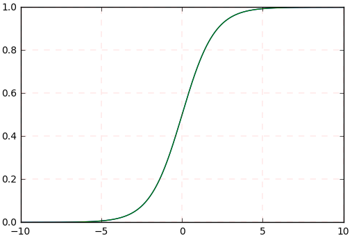
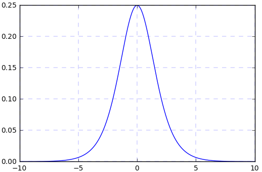
(1) sigmoid 函数曲线 (2) sigmoid 函数的导数曲线
假如我们输入的四个 batch 的数据分布 (或者网络中间某层的输入)(其中黄色线是标准正态分布) 是下图中四个不同颜色的曲线,可以看到:绿色、蓝色、红色曲线的部分值大于 5 或小于 - 5,对应到图 2 中,其导数 (梯度) 值接近于 0,使得在网络反传过程中参数不更新,所以网络训练一直不收敛,训练慢。所以说,网络需要适应不同分布的数据,使得网络训练很慢。
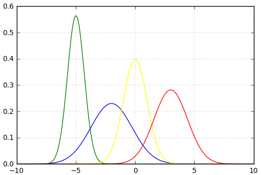
(3) 不同 batch 的数据分布
3.batch norm 引入
二、caffe 中 batch norm 层的源码阅读
1. batch norm
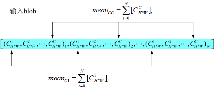
输入 batch norm 层的数据为 [N, C, H, W], 该层计算得到均值为 C 个,方差为 C 个,输出数据为 [N, C, H, W].
<1> 形象点说,均值的计算过程为:
 (1)
(1)
即对 batch 中相同索引的通道数取平均值,所以最终计算得到的均值为 C 个,方差的计算过程与此相同。
<2> batch norm 层的作用:
a. 均值: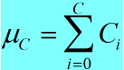 (2)
(2)
b. 方差: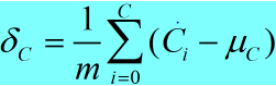 (3)
(3)
c. 归一化: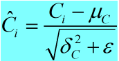 (4)
(4)
<3> batch norm 的反传
源码中提供了反传公式:
1  if Y = (X-mean(X))/(sqrt(var(X)+eps)), then
2  dE(Y)/dX = (dE/dY - mean(dE/dY) - mean(dE/dY \cdot Y) \cdot Y)
3              ./ sqrt(var(X) + eps)
2. caffe 中 batch_norm_layer.cpp 中的 LayerSetUp 函数:
 1 template <typename Dtype>
 2 void BatchNormLayer<Dtype>::LayerSetUp(const vector<Blob<Dtype>*>& bottom,
 3       const vector<Blob<Dtype>*>& top) {
 4   BatchNormParameter param = this->layer_param_.batch_norm_param();
     //读取deploy中moving_average_fraction参数值
 5   moving_average_fraction_ = param.moving_average_fraction();
     //改变量在batch_norm_layer.hpp中的定义为bool use_global_stats_
 6   use_global_stats_ = this->phase_ == TEST;
     //channel在batch_norm_layer.hpp中的定义为int channels_
 7   if (param.has_use_global_stats())
 8     use_global_stats_ = param.use_global_stats();
 9   if (bottom[0]->num_axes() == 1)
10     channels_ = 1;
11   else
12     channels_ = bottom[0]->shape(1);
13   eps_ = param.eps();
14   if (this->blobs_.size() > 0) {
15     LOG(INFO) << "Skipping parameter initialization";
16   } else {
       //blobs的个数为三个,其中:
       //blobs_[0]的尺寸为channels_,保存输入batch中各通道的均值;
       //blobs_[1]的尺寸为channels_,保存输入batch中各通道的方差;
       //blobs_[2]的尺寸为1, 保存moving_average_fraction参数;
       //对上面三个blobs_初始化为0.
17     this->blobs_.resize(3);
18     vector<int> sz;
19     sz.push_back(channels_);
20     this->blobs_[0].reset(new Blob<Dtype>(sz));
21     this->blobs_[1].reset(new Blob<Dtype>(sz));
22     sz[0] = 1;
23     this->blobs_[2].reset(new Blob<Dtype>(sz));
24     for (int i = 0; i < 3; ++i) {
25       caffe_set(this->blobs_[i]->count(), Dtype(0),
26                 this->blobs_[i]->mutable_cpu_data());
27     }
28   }
29   // Mask statistics from optimization by setting local learning rates
30   // for mean, variance, and the bias correction to zero.
31   for (int i = 0; i < this->blobs_.size(); ++i) {
32     if (this->layer_param_.param_size() == i) {
33       ParamSpec* fixed_param_spec = this->layer_param_.add_param();
34       fixed_param_spec->set_lr_mult(0.f);
35     } else {
36       CHECK_EQ(this->layer_param_.param(i).lr_mult(), 0.f)
37           << "Cannot configure batch normalization statistics as layer "
38           << "parameters.";
39     }
40   }
41 }
3. caffe 中 batch_norm_layer.cpp 中的 Reshape 函数:
 1 void BatchNormLayer<Dtype>::Reshape(const vector<Blob<Dtype>*>& bottom,
 2       const vector<Blob<Dtype>*>& top) {
 3   if (bottom[0]->num_axes() >= 1)
 4     CHECK_EQ(bottom[0]->shape(1), channels_);
 5   top[0]->ReshapeLike(*bottom[0]);
     //batch_norm_layer.hpp对如下变量进行了定义:
     //Blob<Dtype> mean_, variance_, temp_, x_norm_;
     //blob<Dtype> batch_sum_multiplier_;
     //blob<Dtype> sum_by_chans_;
     //blob<Dtype> spatial_sum_multiplier_;
 6   vector<int> sz;
 7   sz.push_back(channels_);
     //mean blob和variance blob的尺寸为channel
 8   mean_.Reshape(sz);
 9   variance_.Reshape(sz);
     //temp_ blob和x_norm_ blob的尺寸、数据和输入blob相同
10   temp_.ReshapeLike(*bottom[0]);
11   x_norm_.ReshapeLike(*bottom[0]);
     //sz[0]的值为N,batch_sum_multiplier_ blob的尺寸为N
12   sz[0] = bottom[0]->shape(0);
13   batch_sum_multiplier_.Reshape(sz);
     //spatial_dim = N*C*H*W / C*N = H*W
14   int spatial_dim = bottom[0]->count()/(channels_*bottom[0]->shape(0));
15   if (spatial_sum_multiplier_.num_axes() == 0 ||
16       spatial_sum_multiplier_.shape(0) != spatial_dim) {
17     sz[0] = spatial_dim;
       //spatial_sum_multiplier_的尺寸为H*W, 并且初始化为1
18     spatial_sum_multiplier_.Reshape(sz);
19     Dtype* multiplier_data = spatial_sum_multiplier_.mutable_cpu_data();
20     caffe_set(spatial_sum_multiplier_.count(), Dtype(1), multiplier_data);
21   }
     //numbychans = C*N
22   int numbychans = channels_*bottom[0]->shape(0);
23   if (num_by_chans_.num_axes() == 0 ||
24       num_by_chans_.shape(0) != numbychans) {
25     sz[0] = numbychans;
       //num_by_chans_的尺寸为C*N,并且初始化为1
26     num_by_chans_.Reshape(sz);
27     caffe_set(batch_sum_multiplier_.count(), Dtype(1),
28         batch_sum_multiplier_.mutable_cpu_data());
29   }
30 }
形象点说上面各 blob 变量的尺寸:
mean_和 variance_:元素个数为 channel 的向量
temp_和 x_norm_: 和输入 blob 的尺寸相同,为 N*C*H*W
batch_sum_multiplier_: 元素个数为 N 的向量
spatial_sum_multiplier_: 元素个数为 H*W 的矩阵,并且每个元素的值为 1
num_by_chans_: 元素个数为 C*N 的矩阵,并且每个元素的值为 1
4. caffe 中 batch_norm_layer.cpp 中的 Forward_cpu 函数:
 1 void BatchNormLayer<Dtype>::Forward_cpu(const vector<Blob<Dtype>*>& bottom,
 2     const vector<Blob<Dtype>*>& top) {
 3   const Dtype* bottom_data = bottom[0]->cpu_data();
 4   Dtype* top_data = top[0]->mutable_cpu_data();
     //num = N
 5   int num = bottom[0]->shape(0);
     //spatial_dim = N*C*H*W/N*C = H*W
 6   int spatial_dim = bottom[0]->count()/(bottom[0]->shape(0)*channels_);
 7
 8   if (bottom[0] != top[0]) {
 9     caffe_copy(bottom[0]->count(), bottom_data, top_data);
10   }
11
12   if (use_global_stats_) {
13     // use the stored mean/variance estimates.
       //在测试模式下,scale_factor=1/this->blobs_[2]->cpu_data()[0]
14     const Dtype scale_factor = this->blobs_[2]->cpu_data()[0] == 0 ?
15         0 : 1 / this->blobs_[2]->cpu_data()[0];
       //mean_ blob = scale_factor * this->blobs_[0]->cpu_data()
       //variance_ blob = scale_factor * this_blobs_[1]->cpu_data()
       //因为blobs_变量定义在类中,所以每次调用某一batch norm层时,blobs_[0], blobs_[1], blobs_[2]都会更新
16     caffe_cpu_scale(variance_.count(), scale_factor,
17         this->blobs_[0]->cpu_data(), mean_.mutable_cpu_data());
18     caffe_cpu_scale(variance_.count(), scale_factor,
19         this->blobs_[1]->cpu_data(), variance_.mutable_cpu_data());
20   } else {
21     // compute mean
       //在训练模式下计算一个batch的均值
22     caffe_cpu_gemv<Dtype>(CblasNoTrans, channels_ * num, spatial_dim,
23         1. / (num * spatial_dim), bottom_data,
24         spatial_sum_multiplier_.cpu_data(), 0.,
25         num_by_chans_.mutable_cpu_data());
26     caffe_cpu_gemv<Dtype>(CblasTrans, num, channels_, 1.,
27         num_by_chans_.cpu_data(), batch_sum_multiplier_.cpu_data(), 0.,
28         mean_.mutable_cpu_data());
29   }
30  //由上面两步可以得到:无论是训练,还是测试模式下输入batch的均值
     //对batch中的每个数据减去对应通道的均值
31   // subtract mean
32   caffe_cpu_gemm<Dtype>(CblasNoTrans, CblasNoTrans, num, channels_, 1, 1,
33       batch_sum_multiplier_.cpu_data(), mean_.cpu_data(), 0.,
34       num_by_chans_.mutable_cpu_data());
35   caffe_cpu_gemm<Dtype>(CblasNoTrans, CblasNoTrans, channels_ * num,
36       spatial_dim, 1, -1, num_by_chans_.cpu_data(),
37       spatial_sum_multiplier_.cpu_data(), 1., top_data);
38
39   if (!use_global_stats_) {
       //计算训练模式下的方差
40     // compute variance using var(X) = E((X-EX)^2)
41     caffe_sqr<Dtype>(top[0]->count(), top_data,
42                      temp_.mutable_cpu_data());  // (X-EX)^2
43     caffe_cpu_gemv<Dtype>(CblasNoTrans, channels_ * num, spatial_dim,
44         1. / (num * spatial_dim), temp_.cpu_data(),
45         spatial_sum_multiplier_.cpu_data(), 0.,
46         num_by_chans_.mutable_cpu_data());
47     caffe_cpu_gemv<Dtype>(CblasTrans, num, channels_, 1.,
48         num_by_chans_.cpu_data(), batch_sum_multiplier_.cpu_data(), 0.,
49         variance_.mutable_cpu_data());  // E((X_EX)^2)
50
51     // compute and save moving average
       //在训练阶段,由以上计算步骤可以得到:batch中每个channel的均值和方差
       //blobs_[2] = 1 + blobs_[2]*moving_average_fraction_
       //第一个batch时,blobs_[2]=0, 计算后的blobs_[2] = 1
       //第二个batch时,blobs_[2]=1, 计算后的blobs_[2] = 1 + 1*moving_average_fraction_ = 1.9
52     this->blobs_[2]->mutable_cpu_data()[0] *= moving_average_fraction_;
53     this->blobs_[2]->mutable_cpu_data()[0] += 1;
       //blobs_[0] = 1 * mean_ + moving_average_fraction_ * blobs_[0]
       //其中mean_是本次batch的均值,blobs_[0]是上次batch的均值
54     caffe_cpu_axpby(mean_.count(), Dtype(1), mean_.cpu_data(),
55         moving_average_fraction_, this->blobs_[0]->mutable_cpu_data());
       //m = N*C*H*W/C = N*H*W
56     int m = bottom[0]->count()/channels_;
       //bias_correction_factor = m/m-1
57     Dtype bias_correction_factor = m > 1 ? Dtype(m)/(m-1) : 1;
       //blobs_[1] = bias_correction_factor * variance_ + moving_average_fraction_ * blobs_[1]
58     caffe_cpu_axpby(variance_.count(), bias_correction_factor,
59         variance_.cpu_data(), moving_average_fraction_,
60         this->blobs_[1]->mutable_cpu_data());
61   }
62  //给上一步计算得到的方差加上一个常数eps_,防止方差作为分母在归一化的时候值出现为0的情况,同时开方
63   // normalize variance
64   caffe_add_scalar(variance_.count(), eps_, variance_.mutable_cpu_data());
65   caffe_sqrt(variance_.count(), variance_.cpu_data(),
66              variance_.mutable_cpu_data());
67
68   // replicate variance to input size
     //top_data目前保存的是输入blobs - mean的值,下面几行代码的意思是给每个元素除以对应方差
69   caffe_cpu_gemm<Dtype>(CblasNoTrans, CblasNoTrans, num, channels_, 1, 1,
70       batch_sum_multiplier_.cpu_data(), variance_.cpu_data(), 0.,
71       num_by_chans_.mutable_cpu_data());
72   caffe_cpu_gemm<Dtype>(CblasNoTrans, CblasNoTrans, channels_ * num,
73       spatial_dim, 1, 1., num_by_chans_.cpu_data(),
74       spatial_sum_multiplier_.cpu_data(), 0., temp_.mutable_cpu_data());
75   caffe_div(temp_.count(), top_data, temp_.cpu_data(), top_data);
76   // TODO(cdoersch): The caching is only needed because later in-place layers
77   //                 might clobber the data.  Can we skip this if they won''t?
78   caffe_copy(x_norm_.count(), top_data,
79       x_norm_.mutable_cpu_data());
80 }
caffe_cpu_gemv 的原型为:
1 caffe_cpu_gemv<float>(const CBLAS_TRANSPOSE TransA, const int M, const int N, const float alpha, const float *A, const float *x, const float beta, float *y)实现的功能是矩阵和向量相乘:Y = alpha * A * x + beta * Y
其中,A 矩阵的维度为 M*N, x 向量的维度为 N*1, Y 向量的维度为 M*1.
在训练阶段,forward cpu 函数执行如下步骤:
(1) 均值计算,均值计算的过程如下,分为两步:
<1> 计算 batch 中每个元素的每个 channel 通道的和;
1 caffe_cpu_gemv<Dtype>(CblasNoTrans, channels_ * num, spatial_dim, 1. / (num * spatial_dim), bottom_data, spatial_sum_multiplier_.cpu_data(), 0., num_by_chans_.mutable_cpu_data()); 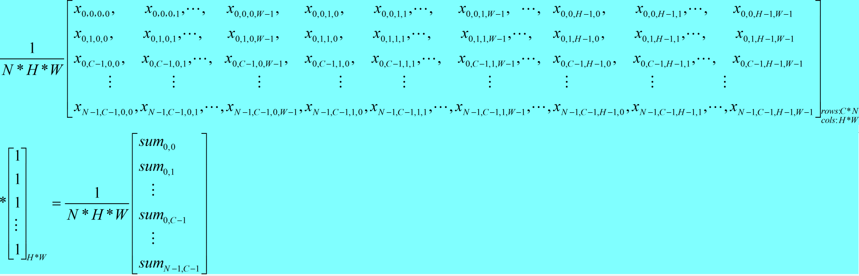
其中:xN-1,C-1,H-1,W-1 表示的含义为:N-1 表示 batch 中的第 N-1 个样本,C-1 表示该样本对应的第 C-1 个通道,H-1 表示该通道中第 H-1 行,W-1 表示该通道中第 W-1 列;
sumN-1,C-1 表示的含义为:batch 中第 N-1 个样本的第 C-1 个通道中所有元素之和。
<2> 计算 batch 中每个通道的均值:
1 caffe_cpu_gemv<Dtype>(CblasTrans, num, channels_, 1., num_by_chans_.cpu_data(), batch_sum_multiplier_.cpu_data(), 0., mean_.mutable_cpu_data()); 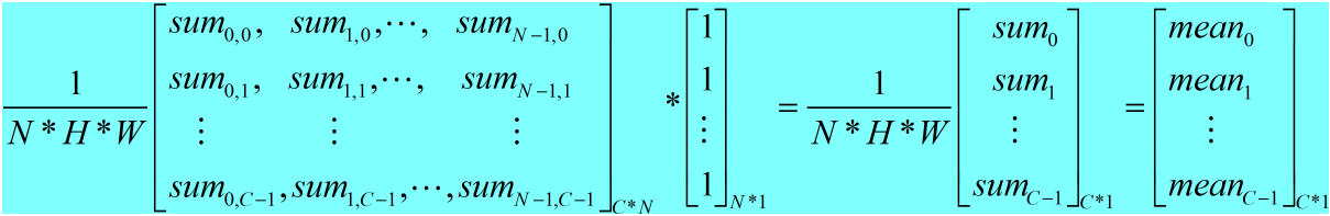
(2) 对 batch 中的每个数据减去其对应通道的均值;
<1> 得到均值矩阵
1 caffe_cpu_gemm<Dtype>(CblasNoTrans, CblasNoTrans, num, channels_, 1, 1, batch_sum_multiplier_.cpu_data(), mean_.cpu_data(), 0., num_by_chans_.mutable_cpu_data()); 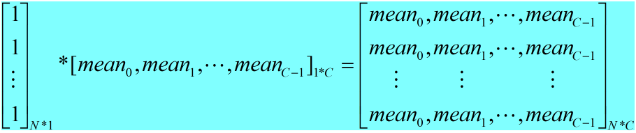
<2> 每个元素减去对应均值
1 caffe_cpu_gemm<Dtype>(CblasNoTrans, CblasNoTrans, channels_ * num, spatial_dim, 1, -1, num_by_chans_.cpu_data(), spatial_sum_multiplier_.cpu_data(), 1., top_data); 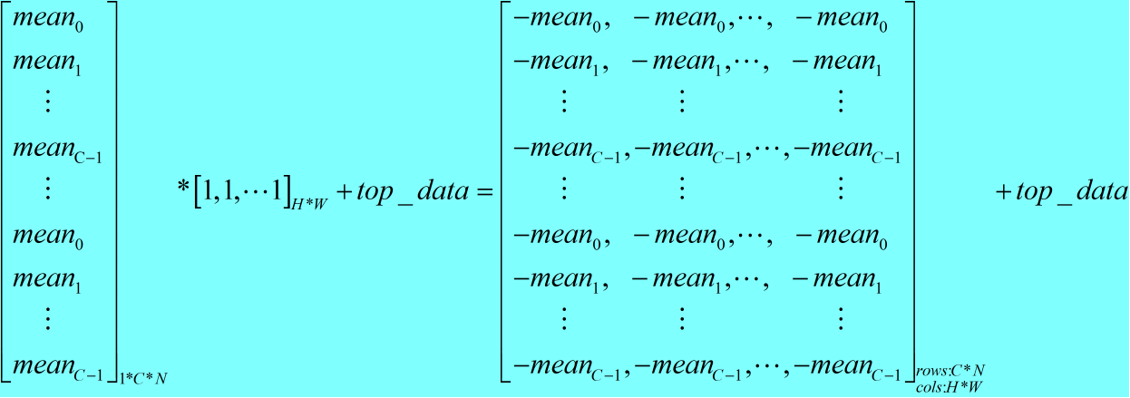
(3) 每个通道的方差计算,计算方式和均值的计算方式相同;
(4) 输入 blob 除以对应方差,得到归一化后的值。
4. caffe 中 batch_norm_layer.cpp 中的 Backward_cpu 函数 (源码中注释的很详细):
 1 void BatchNormLayer<Dtype>::Backward_cpu(const vector<Blob<Dtype>*>& top,
 2     const vector<bool>& propagate_down,
 3     const vector<Blob<Dtype>*>& bottom) {
 4   const Dtype* top_diff;
 5   if (bottom[0] != top[0]) {
 6     top_diff = top[0]->cpu_diff();
 7   } else {
 8     caffe_copy(x_norm_.count(), top[0]->cpu_diff(), x_norm_.mutable_cpu_diff());
 9     top_diff = x_norm_.cpu_diff();
10   }
11   Dtype* bottom_diff = bottom[0]->mutable_cpu_diff();
12   if (use_global_stats_) {
13     caffe_div(temp_.count(), top_diff, temp_.cpu_data(), bottom_diff);
14     return;
15   }
16   const Dtype* top_data = x_norm_.cpu_data();
17   int num = bottom[0]->shape()[0];
18   int spatial_dim = bottom[0]->count()/(bottom[0]->shape(0)*channels_);
19   // if Y = (X-mean(X))/(sqrt(var(X)+eps)), then
20   //
21   // dE(Y)/dX =
22   //   (dE/dY - mean(dE/dY) - mean(dE/dY \cdot Y) \cdot Y)
23   //     ./ sqrt(var(X) + eps)
24   //
25   // where \cdot and ./ are hadamard product and elementwise division,
26   // respectively, dE/dY is the top diff, and mean/var/sum are all computed
27   // along all dimensions except the channels dimension.  In the above
28   // equation, the operations allow for expansion (i.e. broadcast) along all
29   // dimensions except the channels dimension where required.
30
31   // sum(dE/dY \cdot Y)
32   caffe_mul(temp_.count(), top_data, top_diff, bottom_diff);
33   caffe_cpu_gemv<Dtype>(CblasNoTrans, channels_ * num, spatial_dim, 1.,
34       bottom_diff, spatial_sum_multiplier_.cpu_data(), 0.,
35       num_by_chans_.mutable_cpu_data());
36   caffe_cpu_gemv<Dtype>(CblasTrans, num, channels_, 1.,
37       num_by_chans_.cpu_data(), batch_sum_multiplier_.cpu_data(), 0.,
38       mean_.mutable_cpu_data());
39
40   // reshape (broadcast) the above
41   caffe_cpu_gemm<Dtype>(CblasNoTrans, CblasNoTrans, num, channels_, 1, 1,
42       batch_sum_multiplier_.cpu_data(), mean_.cpu_data(), 0.,
43       num_by_chans_.mutable_cpu_data());
44   caffe_cpu_gemm<Dtype>(CblasNoTrans, CblasNoTrans, channels_ * num,
45       spatial_dim, 1, 1., num_by_chans_.cpu_data(),
46       spatial_sum_multiplier_.cpu_data(), 0., bottom_diff);
47
48   // sum(dE/dY \cdot Y) \cdot Y
49   caffe_mul(temp_.count(), top_data, bottom_diff, bottom_diff);
50
51   // sum(dE/dY)-sum(dE/dY \cdot Y) \cdot Y
52   caffe_cpu_gemv<Dtype>(CblasNoTrans, channels_ * num, spatial_dim, 1.,
53       top_diff, spatial_sum_multiplier_.cpu_data(), 0.,
54       num_by_chans_.mutable_cpu_data());
55   caffe_cpu_gemv<Dtype>(CblasTrans, num, channels_, 1.,
56       num_by_chans_.cpu_data(), batch_sum_multiplier_.cpu_data(), 0.,
57       mean_.mutable_cpu_data());
58   // reshape (broadcast) the above to make
59   // sum(dE/dY)-sum(dE/dY \cdot Y) \cdot Y
60   caffe_cpu_gemm<Dtype>(CblasNoTrans, CblasNoTrans, num, channels_, 1, 1,
61       batch_sum_multiplier_.cpu_data(), mean_.cpu_data(), 0.,
62       num_by_chans_.mutable_cpu_data());
63   caffe_cpu_gemm<Dtype>(CblasNoTrans, CblasNoTrans, num * channels_,
64       spatial_dim, 1, 1., num_by_chans_.cpu_data(),
65       spatial_sum_multiplier_.cpu_data(), 1., bottom_diff);
66
67   // dE/dY - mean(dE/dY)-mean(dE/dY \cdot Y) \cdot Y
68   caffe_cpu_axpby(temp_.count(), Dtype(1), top_diff,
69       Dtype(-1. / (num * spatial_dim)), bottom_diff);
70
71   // note: temp_ still contains sqrt(var(X)+eps), computed during the forward
72   // pass.
73   caffe_div(temp_.count(), bottom_diff, temp_.cpu_data(), bottom_diff);
74 }
note: 可以看到,caffe 中:
<a> 通过两个 caffe_cpu_gemv 函数将一个矩阵变为一个向量,例如:
caffe_cpu_gemv: [(C*N)*(H*W)] * [(H*W) * 1 ] = C*N;
caffe_cpu_gemv: [C*N] * [N*1] = C*1
<b> 通过两个 caffe_cpu_gemm 函数将一个向量变为一个矩阵。
caffe_cpu_gemm 和上面的过程刚好是反过来。
原文出处:https://www.cnblogs.com/liangx-img/p/11726371.html

Batch Norm、Layer Norm、Weight Norm与SELU
加速网络收敛——BN、LN、WN与selu
自Batch Norm出现之后,Layer Norm和Weight Norm作为Batch Norm的变体相继出现。最近又出来一个很”简单”的激活函数Selu,能够实现automatic rescale and shift。这些结构都是为了保证网络能够堆叠的更深的基本条件之一。除了这四种,还有highway network与resnet。
Batch Norm
BN对某一层激活值做batch维度的归一化,也就是对于每个batch,该层相应的output位置归一化所使用的mean和variance都是一样的。
- BN的学习参数包含rescale和shift两个参数;训练的时候不断更新这两个参数和moving average mean and variance
- BN在单独的层级之间使用比较方便,比如CNN
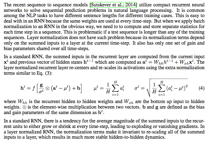
- 像RNN这样unroll之后层数不定,直接用BN不太方便,需要对每一层(每个time step)做BN,并保留每一层的mean和variance。不过由于RNN输入不定长(time step长度不定),可能会有validation或test的time step比train set里面的任何数据都长,因此会造成mean和variance不存在的情况。针对这个情况,需要对每个time step独立做统计。在BN-LSTM中是这么做的:Generalizing the model to sequences longer than those seen during training is straightforward thanks to the rapid convergence of the activations to their steady-state distributions (cf. Figure 5). For our experiments we estimate the population statistics separately for each timestep 1, . . . , Tmax where Tmax is the length of the longest training sequence. When at test time we need to generalize beyond Tmax, we use the population statistic of time Tmax for all time steps beyond it. During training we estimate the statistics across the minibatch, independently for each timestep. At test time we use estimates obtained by averaging the minibatch estimates over the training set.当然,也可以只对输入-隐层进行BN,或者stack RNN中同一个time step的不同层之间做BN
- BN会引入噪声(因为是mini batch而不是整个training set),所以对于噪声敏感的方法(如RL)不太适用
BN算法思路如下(注意training和inference时候的区别)。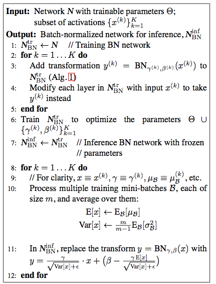
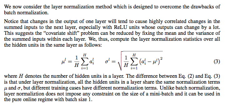
Layer Norm
LN也是对输出归一化的。LN也是为了消除各层的covariate shift,加快收敛速度。LN相对于BN就简单多了。
- 它在training和inference时没有区别,只需要对当前隐藏层计算mean and variance就行
- 不需要保存每层的moving average mean and variance
- 不受batch size的限制,可以通过online learning的方式一条一条的输入训练数据
- LN可以方便的在RNN中使用
- LN增加了gain和bias作为学习的参数,μ和σ分别是该layer的隐层维度的均值和方差
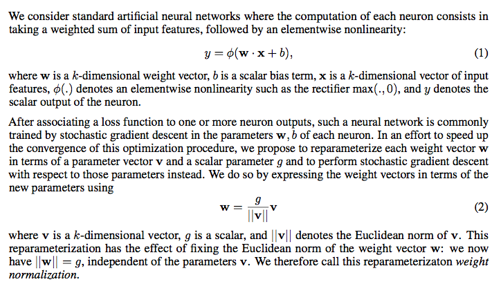
Weight Norm
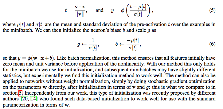
WN是使用参数重写(reparameterization weight normalization)的方法来做归一化的。哪里有weight,哪里就可以用WN来归一化。WN也是用来加速收敛的。通过对weight进行normalization,可以保证在梯度回传的时候,如果梯度越noisy(梯度越大),v的norm就越大,那么g/||v||就越小,从而就会抑制梯度。做到了梯度的自稳定(self-stabilize)。
-
与LN稍不一样,WN只有gain这一个学习参数
-
前向传播时,BN就是简单的normalization
- 梯度回传的时候,会对梯度做自稳定
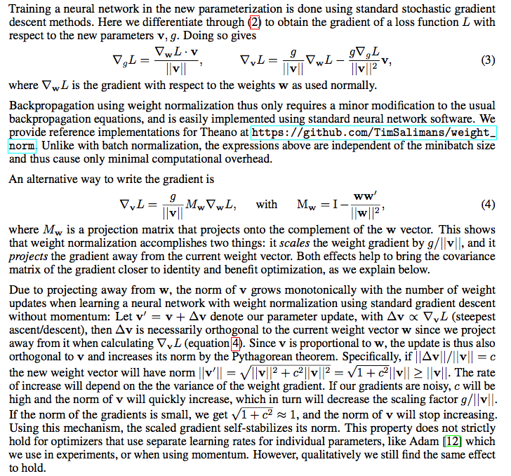
- 论文里提到了WN能够让learning rate自适应/自稳定
If the learning rate is too large, the norm of the unnormalized weights grows quickly until an appropriate effective learning rate is reached. Once the norm of the weights has grown large with respect to the norm of the updates, the effective learning rate stabilizes.
- WN与BN一样,只不过BN直接从输出角度出发,WN从weight角度出发
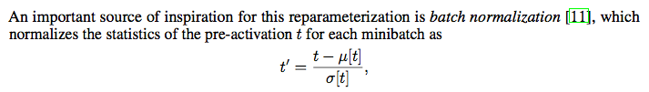
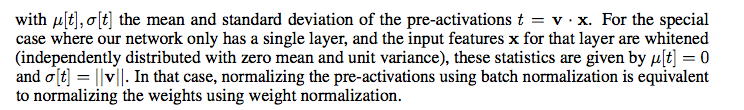
- 注意WN的初始化,需要用第一个minibatch的均值和方差来初始化g和b。
- Mean-only BN
考虑到BN并不能保证参数v的协方差矩阵为单位矩阵,也就是BN不能保证激活值与v独立。而WN能做到,因此可以结合WN与BN,此时的BN经过修改,只进行去均值操作。
selu
最理想的结果就是让每一层输出的激活值为零均值、单位方差,从而能够使得张量在传播的过程当中,不会出现covariant shift,保证回传梯度的稳定性,不会有梯度爆炸或弥散的问题。selu能够很好的实现automatically shift and rescale neuron activations towards zero mean and unit variance without explicit normalization like what batch normalization technique does.
并且可以参考References中的Selus与Leaky Relu以及Relu之间的对比。selu 推荐用在大训练样本的数据集上。
References
Weight Normalization: A Simple Reparameterization to Accelerate Training of Deep Neural Networks
Batch Normalization: Accelerating Deep Network Training by Reducing Internal Covariate Shift
RECURRENT BATCH NORMALIZATION
Layer Normalization
深度学习加速策略BN、WN和LN的联系与区别,各自的优缺点和适用的场景?
SELUs (scaled exponential linear units) - Visualized and Histogramed Comparisons among ReLU and Leaky ReLU
引爆机器学习圈:「自归一化神经网络」提出新型激活函数SELU

bn两个参数的计算以及layer norm、instance norm、group norm
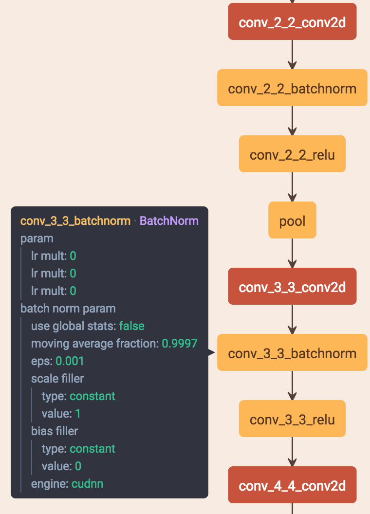
bn一般就在conv之后并且后面再接relu
1.如果输入feature map channel是6,bn的gamma beta个数是多少个?
6个。
2.bn的缺点:
BN会受到batchsize大小的影响。如果batchsize太小,算出的均值和方差就会不准确,如果太大,显存又可能不够用。
3.训练和测试时一般不一样,一般都是训练的时候在训练集上通过滑动平均预先计算好平均-mean,和方差-variance参数,在测试的时候,不再计算这些值,而是直接调用这些预计算好的来用,但是,当训练数据和测试数据分布有差别是时,训练机上预计算好的数据并不能代表测试数据,这就导致在训练,验证,测试这三个阶段存inconsistency
4.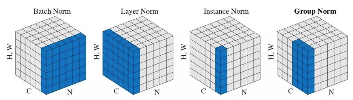
batch norm:在一个batch里所有样本的feature map的同一个channel上进行norm,归一化维度为[N,H,W]
layer norm:在每个样本所有的channel上进行norm,归一化的维度为[C,H,W]
instance norm:在每个样本每个channel上进行norm,归一化的维度为[H,W]
group norm:将channel方向分group,然后每个group内做归一化,算(C//G)*H*W的均值,GN的极端情况就是LN和I N
GG 表示分组的数量, 是一个预定义的超参数(一般选择 G=32G=32). C/GC/G 是每个组的通道数, 第二个等式条件表示对处于同一组的像素计算均值和标准差. 最终得到的形状为 N×(C/G)
延伸问题:这个group norm怎么去求?
http://www.dataguru.cn/article-13318-1.html
https://blog.csdn.net/qq_14845119/article/details/79702040
1.跨卡同步的BN能有效提升性能
其实这是可以理解的,毕竟这样bn进行的batch size增大,batch size越大,bn对性能提升越好
2.训练、测试的bn不同
在训练的时候用移动平均(类似于momentum)的方式更新batch mean和variance,训练完毕,得到一个相对比较稳定的mean和variance,存在模型中。
测试的时候,就直接用模型中的均值和方差进行计算。
这个存储的bn参数是通过移动平均法得到的:
当前mean = 0.1 * 当前mean + 0.9 * 以前的mean
var同理
今天关于将 np.linalg.norm() (python) 应用于 2d numpy 数组的每个元素和给定值的最快方法是什么?的介绍到此结束,谢谢您的阅读,有关.NET norm —— 轻量级 orm 开发框架 norm、batch norm 理解和 caffe 中 batch norm 层阅读、Batch Norm、Layer Norm、Weight Norm与SELU、bn两个参数的计算以及layer norm、instance norm、group norm等更多相关知识的信息可以在本站进行查询。
本文标签:


