在本文中,我们将给您介绍关于Pythonnumpy模块-diagflat()实例源码的详细内容,并且为您解答python中numpy模块的相关问题,此外,我们还将为您提供关于Jupyter中的Nump
在本文中,我们将给您介绍关于Python numpy 模块-diagflat() 实例源码的详细内容,并且为您解答python中numpy模块的相关问题,此外,我们还将为您提供关于Jupyter 中的 Numpy 在打印时出错(Python 版本 3.8.8):TypeError: 'numpy.ndarray' object is not callable、numpy.random.random & numpy.ndarray.astype & numpy.arange、numpy.ravel()/numpy.flatten()/numpy.squeeze()、Numpy:数组创建 numpy.arrray() , numpy.arange()、np.linspace ()、数组基本属性的知识。
本文目录一览:- Python numpy 模块-diagflat() 实例源码(python中numpy模块)
- Jupyter 中的 Numpy 在打印时出错(Python 版本 3.8.8):TypeError: 'numpy.ndarray' object is not callable
- numpy.random.random & numpy.ndarray.astype & numpy.arange
- numpy.ravel()/numpy.flatten()/numpy.squeeze()
- Numpy:数组创建 numpy.arrray() , numpy.arange()、np.linspace ()、数组基本属性
 实例源码(python中numpy模块)")
Python numpy 模块-diagflat() 实例源码(python中numpy模块)
Python numpy 模块,diagflat() 实例源码
我们从Python开源项目中,提取了以下17个代码示例,用于说明如何使用numpy.diagflat()。
- def train(self):
- X = self.train_x
- y = self.train_y
- # include intercept
- beta = np.zeros((self.p+1, 1))
- iter_times = 0
- while True:
- e_X = np.exp(X @ beta)
- # N x 1
- self.P = e_X / (1 + e_X)
- # W is a vector
- self.W = (self.P * (1 - self.P)).flatten()
- # X.T * W equal (X.T @ diagflat(W)).diagonal()
- beta = beta + self.math.pinv((X.T * self.W) @ X) @ X.T @ (y - self.P)
- iter_times += 1
- if iter_times > self.max_iter:
- break
- self.beta_hat = beta
- def latent_correlation(self):
- """Compute correlation matrix among latent features.
- This computes the generalization of Pearson''s correlation to discrete
- data. Let I(X;Y) be the mutual information. Then define correlation as
- rho(X,Y) = sqrt(1 - exp(-2 I(X;Y)))
- Returns:
- A [V,V]-shaped numpy array of feature-feature correlations.
- """
- logger.debug(''computing latent correlation'')
- V, E, M, R = self._VEMR
- edge_probs = self._edge_probs
- vert_probs = self._vert_probs
- result = np.zeros([V, V], np.float32)
- for root in range(V):
- messages = np.empty([V, M])
- program = make_propagation_program(self._tree.tree_grid, root)
- for op, v, v2, e in program:
- if op == OP_ROOT:
- # Initialize correlation at this node.
- messages[v, :, :] = np.diagflat(vert_probs[v, :])
- elif op == OP_OUT:
- # Propagate correlation outward from parent to v.
- trans = edge_probs[e, :]
- if v > v2:
- trans = trans.T
- messages[v, :] = np.dot( #
- trans / vert_probs[v2, np.newaxis, :],
- messages[v2, :])
- for v in range(V):
- result[root, v] = correlation(messages[v, :])
- return result
- def train(self):
- super().train()
- sigma = self.Sigma_hat
- D_, U = LA.eigh(sigma)
- D = np.diagflat(D_)
- self.A = np.power(LA.pinv(D), 0.5) @ U.T
- def train(self):
- super().train()
- W = self.Sigma_hat
- # prior probabilities (K,1)
- Pi = self.Pi
- # class centroids (K,p)
- Mu = self.Mu
- p = self.p
- # the number of class
- K = self.n_class
- # the dimension you want
- L = self.L
- # Mu is (K,p) matrix,Pi is (K,1)
- mu = np.sum(Pi * Mu, axis=0)
- B = np.zeros((p, p))
- for k in range(K):
- # vector @ vector equal scalar,use vector[:,None] to transform to matrix
- # vec[:,None] equal to vec.reshape((1,vec.shape[0]))
- B = B + Pi[k]*((Mu[k] - mu)[:, None] @ ((Mu[k] - mu)[None, :]))
- # Be careful,the `eigh` method get the eigenvalues in ascending,which is opposite to R.
- Dw, Uw = LA.eigh(W)
- # reverse the Dw_ and Uw
- Dw = Dw[::-1]
- Uw = np.fliplr(Uw)
- W_half = self.math.pinv(np.diagflat(Dw**0.5) @ Uw.T)
- B_star = W_half.T @ B @ W_half
- D_, V = LA.eigh(B_star)
- # reverse V
- V = np.fliplr(V)
- # overwrite `self.A` so that we can reuse `predict` method define in parent class
- self.A = np.zeros((L, p))
- for l in range(L):
- self.A[l, :] = W_half @ V[:, l]
- def _update_(U, D, d, lambda_):
- """Go from u(n) to u(n+1)."""
- I = np.identity(3)
- m = U.T.dot(d)
- p = (I - U.dot(U.T)).dot(d)
- p_norm = np.linalg.norm(p)
- # Make p and m column vectors
- p = p[np.newaxis].T
- m = m[np.newaxis].T
- U_left = np.hstack((U, p/p_norm))
- Q = np.hstack((lambda_ * D, m))
- Q = np.vstack((Q, [0, 0, p_norm]))
- # SVD
- U_right, D_new, V_left = np.linalg.svd(Q)
- # Get rid of the smallest eigenvalue
- D_new = D_new[0:2]
- D_new = np.diagflat(D_new)
- U_right = U_right[:, 0:2]
- return U_left.dot(U_right), D_new
- def rosenberger(datax, dataY, dataZ, lambda_):
- """
- Separate P and non-P wavefield from 3-component data.
- Return a two set of 3-component traces.
- """
- # Construct the data matrix
- A = np.vstack((dataZ, datax, dataY))
- # SVD of the first 3 samples:
- U, V = np.linalg.svd(A[:, 0:3])
- # Get rid of the smallest eigenvalue
- D = D[0:2]
- D = np.diagflat(D)
- U = U[:, 0:2]
- save_U = np.zeros(len(datax))
- save_U[0] = abs(U[0, 0])
- Dp = np.zeros((3, len(datax)))
- Ds = np.zeros((3, len(datax)))
- Dp[:, 0] = abs(U[0, 0]) * A[:, 2]
- Ds[:, 0] = (1 - abs(U[0, 0])) * A[:, 2]
- # Loop over all the values
- for i in range(1, A.shape[1]):
- d = A[:, i]
- U, D = _update_(U, lambda_)
- Dp[:, i] = abs(U[0, 0]) * d
- Ds[:, i] = (1-abs(U[0, 0])) * d
- save_U[i] = abs(U[0, 0])
- return Dp, Ds, save_U
- def eye(n): return diagflat(ones(n))
- def diagflat(a, k=0):
- if isinstance(a, garray): return a.diagflat(k)
- else: return numpy.diagflat(a,k)
- def diagflat(self, k=0):
- if self.ndim!=1: return self.ravel().diagflat(k)
- if k!=0: raise NotImplementedError(''k!=0 for garray.diagflat'')
- selfSize = self.size
- ret = zeros((selfSize, selfSize))
- ret.ravel()[:-1].reshape((selfSize-1, selfSize+1))[:, 0] = self[:-1]
- if selfSize!=0: ret.ravel()[-1] = self[-1]
- return ret
- def diagonal(self):
- if self.ndim==1: return self.diagflat()
- if self.ndim==2:
- if self.shape[0] > self.shape[1]: return self[:self.shape[1]].diagonal()
- if self.shape[1] > self.shape[0]: return self[:, :self.shape[0]].diagonal()
- return self.ravel()[::self.shape[0]+1]
- raise NotImplementedError(''garray.diagonal for arrays with ndim other than 1 or 2.'')
- def eye(n): return diagflat(ones(n))
- def diagflat(self, 0] = self[:-1]
- if selfSize!=0: ret.ravel()[-1] = self[-1]
- return ret
- def diagonal(self):
- if self.ndim==1: return self.diagflat()
- if self.ndim==2:
- if self.shape[0] > self.shape[1]: return self[:self.shape[1]].diagonal()
- if self.shape[1] > self.shape[0]: return self[:, :self.shape[0]].diagonal()
- return self.ravel()[::self.shape[0]+1]
- raise NotImplementedError(''garray.diagonal for arrays with ndim other than 1 or 2.'')
- def fit(self, dHdl):
- """
- Compute free energy differences between each state by integrating
- dHdl across lambda values.
- Parameters
- ----------
- dHdl : DataFrame
- dHdl[n,k] is the potential energy gradient with respect to lambda
- for each configuration n and lambda k.
- """
- # sort by state so that rows from same state are in contiguous blocks,
- # and adjacent states are next to each other
- dHdl = dHdl.sort_index(level=dHdl.index.names[1:])
- # obtain the mean and variance of the mean for each state
- # variance calculation assumes no correlation between points
- # used to calculate mean
- means = dHdl.mean(level=dHdl.index.names[1:])
- variances = np.square(dHdl.sem(level=dHdl.index.names[1:]))
- # obtain vector of delta lambdas between each state
- dl = means.reset_index()[means.index.names[:]].diff().iloc[1:].values
- # apply trapezoid rule to obtain DF between each adjacent state
- deltas = (dl * (means.iloc[:-1].values + means.iloc[1:].values)/2).sum(axis=1)
- d_deltas = (dl**2 * (variances.iloc[:-1].values + variances.iloc[1:].values)/4).sum(axis=1)
- # build matrix of deltas between each state
- adelta = np.zeros((len(deltas)+1, len(deltas)+1))
- ad_delta = np.zeros_like(adelta)
- for j in range(len(deltas)):
- out = []
- dout = []
- for i in range(len(deltas) - j):
- out.append(deltas[i] + deltas[i+1:i+j+1].sum())
- dout.append(d_deltas[i] + d_deltas[i+1:i+j+1].sum())
- adelta += np.diagflat(np.array(out), k=j+1)
- ad_delta += np.diagflat(np.array(dout), k=j+1)
- # yield standard delta_f_ free energies between each state
- self.delta_f_ = pd.DataFrame(adelta - adelta.T,
- columns=means.index.values,
- index=means.index.values)
- # yield standard deviation d_delta_f_ between each state
- self.d_delta_f_ = pd.DataFrame(np.sqrt(ad_delta + ad_delta.T),
- columns=variances.index.values,
- index=variances.index.values)
- self.states_ = means.index.values.tolist()
- return self
- def simplex_project(y, infinitesimal):
- # 1-D vector version
- # D = len(y)
- # u = np.sort(y)[::-1]
- # x_tmp = (1. - np.cumsum(u)) / np.arange(1,D+1)
- # lmd = x_tmp[np.sum(u + x_tmp > 0) - 1]
- # return np.maximum(y + lmd,0)
- n, d = y.shape
- x = np.fliplr(np.sort(y, axis=1))
- x_tmp = np.dot((np.cumsum(x, axis=1) + (d * infinitesimal - 1.)), np.diagflat(1. / np.arange(1, d + 1)))
- lmd = x_tmp[np.arange(n), np.sum(x > x_tmp, axis=1) - 1]
- return np.maximum(y - lmd[:, np.newaxis], 0) + infinitesimal
- def JCB(A,b,N=25,x=None):
- if x is None:
- x = zeros(len(A[0]))
- D = diag(A)
- R = A - diagflat(D)
- for i in range(N):
- x = (b - dot(R,x))/D
- pprint(x)
- return x
- def diagflat(a,k)
:TypeError: 'numpy.ndarray' object is not callable")
Jupyter 中的 Numpy 在打印时出错(Python 版本 3.8.8):TypeError: 'numpy.ndarray' object is not callable
如何解决Jupyter 中的 Numpy 在打印时出错(Python 版本 3.8.8):TypeError: ''numpy.ndarray'' object is not callable?
晚安, 尝试打印以下内容时,我在 jupyter 中遇到了 numpy 问题,并且得到了一个 错误: 需要注意的是python版本是3.8.8。 我先用 spyder 测试它,它运行正确,它给了我预期的结果
使用 Spyder:
import numpy as np
    for i in range (5):
        n = np.random.rand ()
    print (n)
Results
0.6604903457995978
0.8236300859753154
0.16067650689842816
0.6967868357083673
0.4231597934445466
现在有了 jupyter
import numpy as np
    for i in range (5):
        n = np.random.rand ()
    print (n)
-------------------------------------------------- ------
TypeError Traceback (most recent call last)
<ipython-input-78-0c6a801b3ea9> in <module>
       2 for i in range (5):
       3 n = np.random.rand ()
---->  4 print (n)

       TypeError: ''numpy.ndarray'' object is not callable
感谢您对我如何在 Jupyter 中解决此问题的帮助。
非常感谢您抽出宝贵时间。
阿特,约翰”
解决方法
暂无找到可以解决该程序问题的有效方法,小编努力寻找整理中!
如果你已经找到好的解决方法,欢迎将解决方案带上本链接一起发送给小编。
小编邮箱:dio#foxmail.com (将#修改为@)

numpy.random.random & numpy.ndarray.astype & numpy.arange
今天看到这样一句代码:
xb = np.random.random((nb, d)).astype(''float32'') #创建一个二维随机数矩阵(nb行d列)
xb[:, 0] += np.arange(nb) / 1000. #将矩阵第一列的每个数加上一个值要理解这两句代码需要理解三个函数
1、生成随机数
numpy.random.random(size=None)
size为None时,返回float。
size不为None时,返回numpy.ndarray。例如numpy.random.random((1,2)),返回1行2列的numpy数组
2、对numpy数组中每一个元素进行类型转换
numpy.ndarray.astype(dtype)
返回numpy.ndarray。例如 numpy.array([1, 2, 2.5]).astype(int),返回numpy数组 [1, 2, 2]
3、获取等差数列
numpy.arange([start,]stop,[step,]dtype=None)
功能类似python中自带的range()和numpy中的numpy.linspace
返回numpy数组。例如numpy.arange(3),返回numpy数组[0, 1, 2]
/numpy.flatten()/numpy.squeeze()")
numpy.ravel()/numpy.flatten()/numpy.squeeze()
numpy.ravel(a, order=''C'')
Return a flattened array
numpy.chararray.flatten(order=''C'')
Return a copy of the array collapsed into one dimension
numpy.squeeze(a, axis=None)
Remove single-dimensional entries from the shape of an array.
相同点: 将多维数组 降为 一维数组
不同点:
ravel() 返回的是视图(view),意味着改变元素的值会影响原始数组元素的值;
flatten() 返回的是拷贝,意味着改变元素的值不会影响原始数组;
squeeze()返回的是视图(view),仅仅是将shape中dimension为1的维度去掉;
ravel()示例:
 1 import matplotlib.pyplot as plt
 2 import numpy as np
 3
 4 def log_type(name,arr):
 5     print("数组{}的大小:{}".format(name,arr.size))
 6     print("数组{}的维度:{}".format(name,arr.shape))
 7     print("数组{}的维度:{}".format(name,arr.ndim))
 8     print("数组{}元素的数据类型:{}".format(name,arr.dtype))
 9     #print("数组:{}".format(arr.data))
10
11 a = np.floor(10*np.random.random((3,4)))
12 print(a)
13 log_type(''a'',a)
14
15 a1 = a.ravel()
16 print("a1:{}".format(a1))
17 log_type(''a1'',a1)
18 a1[2] = 100
19
20 print(a)
21 log_type(''a'',a)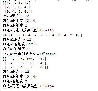
flatten()示例
 1 import matplotlib.pyplot as plt
 2 import numpy as np
 3
 4 def log_type(name,arr):
 5     print("数组{}的大小:{}".format(name,arr.size))
 6     print("数组{}的维度:{}".format(name,arr.shape))
 7     print("数组{}的维度:{}".format(name,arr.ndim))
 8     print("数组{}元素的数据类型:{}".format(name,arr.dtype))
 9     #print("数组:{}".format(arr.data))
10
11 a = np.floor(10*np.random.random((3,4)))
12 print(a)
13 log_type(''a'',a)
14
15 a1 = a.flatten()
16 print("修改前a1:{}".format(a1))
17 log_type(''a1'',a1)
18 a1[2] = 100
19 print("修改后a1:{}".format(a1))
20
21 print("a:{}".format(a))
22 log_type(''a'',a)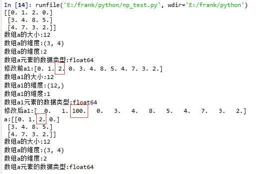
squeeze()示例:
1. 没有single-dimensional entries的情况
 1 import matplotlib.pyplot as plt
 2 import numpy as np
 3
 4 def log_type(name,arr):
 5     print("数组{}的大小:{}".format(name,arr.size))
 6     print("数组{}的维度:{}".format(name,arr.shape))
 7     print("数组{}的维度:{}".format(name,arr.ndim))
 8     print("数组{}元素的数据类型:{}".format(name,arr.dtype))
 9     #print("数组:{}".format(arr.data))
10
11 a = np.floor(10*np.random.random((3,4)))
12 print(a)
13 log_type(''a'',a)
14
15 a1 = a.squeeze()
16 print("修改前a1:{}".format(a1))
17 log_type(''a1'',a1)
18 a1[2] = 100
19 print("修改后a1:{}".format(a1))
20
21 print("a:{}".format(a))
22 log_type(''a'',a)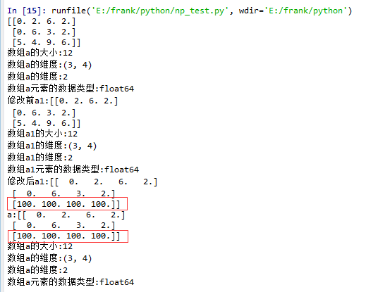
从结果中可以看到,当没有single-dimensional entries时,squeeze()返回额数组对象是一个view,而不是copy。
2. 有single-dimentional entries 的情况
 1 import matplotlib.pyplot as plt
 2 import numpy as np
 3
 4 def log_type(name,arr):
 5     print("数组{}的大小:{}".format(name,arr.size))
 6     print("数组{}的维度:{}".format(name,arr.shape))
 7     print("数组{}的维度:{}".format(name,arr.ndim))
 8     print("数组{}元素的数据类型:{}".format(name,arr.dtype))
 9     #print("数组:{}".format(arr.data))
10
11 a = np.floor(10*np.random.random((1,3,4)))
12 print(a)
13 log_type(''a'',a)
14
15 a1 = a.squeeze()
16 print("修改前a1:{}".format(a1))
17 log_type(''a1'',a1)
18 a1[2] = 100
19 print("修改后a1:{}".format(a1))
20
21 print("a:{}".format(a))
22 log_type(''a'',a)
 , numpy.arange()、np.linspace ()、数组基本属性")
Numpy:数组创建 numpy.arrray() , numpy.arange()、np.linspace ()、数组基本属性
一、Numpy数组创建
part 1:np.linspace(起始值,终止值,元素总个数
import numpy as np
''''''
numpy中的ndarray数组
''''''

ary = np.array([1, 2, 3, 4, 5])
print(ary)
ary = ary * 10
print(ary)

''''''
ndarray对象的创建
''''''
# 创建二维数组
# np.array([[],[],...])
a = np.array([[1, 2, 3, 4], [5, 6, 7, 8]])
print(a)

# np.arange(起始值, 结束值, 步长(默认1))
b = np.arange(1, 10, 1)
print(b)

print("-------------np.zeros(数组元素个数, dtype=''数组元素类型'')-----")
# 创建一维数组:
c = np.zeros(10)
print(c, ''; c.dtype:'', c.dtype)

# 创建二维数组:
print(np.zeros ((3,4)))

print("----------np.ones(数组元素个数, dtype=''数组元素类型'')--------")
# 创建一维数组:
d = np.ones(10, dtype=''int64'')
print(d, ''; d.dtype:'', d.dtype)

# 创建三维数组:
print(np.ones( (2,3,4), dtype=np.int32 ))
# 打印维度
print(np.ones( (2,3,4), dtype=np.int32 ).ndim)  # 返回:3(维)
结果图:

part 2 :np.linspace ( 起始值,终止值,元素总个数)
import numpy as np
a = np.arange( 10, 30, 5 )

b = np.arange( 0, 2, 0.3 )

c = np.arange(12).reshape(4,3)

d = np.random.random((2,3))  # 取-1到1之间的随机数,要求设置为诶2行3列的结构

print(a)
print(b)
print(c)
print(d)

print("-----------------")
from numpy import pi
print(np.linspace( 0, 2*pi, 100 ))

print("-------------np.linspace(起始值,终止值,元素总个数)------------------")
print(np.sin(np.linspace( 0, 2*pi, 100 )))
结果图:

二、Numpy的ndarray对象属性:
数组的结构:array.shape
数组的维度:array.ndim
元素的类型:array.dtype
数组元素的个数:array.size
数组的索引(下标):array[0]
''''''
数组的基本属性
''''''
import numpy as np
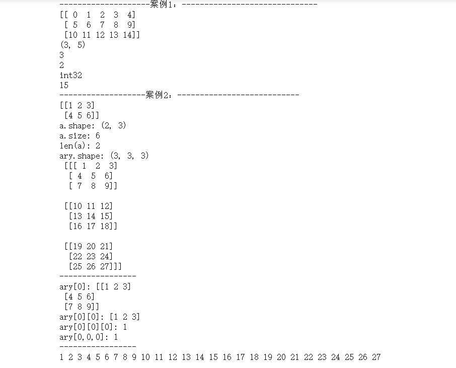
print("--------------------案例1:------------------------------")
a = np.arange(15).reshape(3, 5)
print(a)
print(a.shape) # 打印数组结构
print(len(a)) # 打印有多少行
print(a.ndim) # 打印维度
print(a.dtype) # 打印a数组内的元素的数据类型
# print(a.dtype.name)
print(a.size) # 打印数组的总元素个数
print("-------------------案例2:---------------------------")
a = np.array([[1, 2, 3], [4, 5, 6]])
print(a)
# 测试数组的基本属性
print(''a.shape:'', a.shape)
print(''a.size:'', a.size)
print(''len(a):'', len(a))
# a.shape = (6, ) # 此格式可将原数组结构变成1行6列的数据结构
# print(a, ''a.shape:'', a.shape)
# 数组元素的索引
ary = np.arange(1, 28)
ary.shape = (3, 3, 3) # 创建三维数组
print("ary.shape:",ary.shape,"\n",ary )
print("-----------------")
print(''ary[0]:'', ary[0])
print(''ary[0][0]:'', ary[0][0])
print(''ary[0][0][0]:'', ary[0][0][0])
print(''ary[0,0,0]:'', ary[0, 0, 0])
print("-----------------")
# 遍历三维数组:遍历出数组里的每个元素
for i in range(ary.shape[0]):
for j in range(ary.shape[1]):
for k in range(ary.shape[2]):
print(ary[i, j, k], end='' '')
结果图:
关于Python numpy 模块-diagflat() 实例源码和python中numpy模块的介绍已经告一段落,感谢您的耐心阅读,如果想了解更多关于Jupyter 中的 Numpy 在打印时出错(Python 版本 3.8.8):TypeError: 'numpy.ndarray' object is not callable、numpy.random.random & numpy.ndarray.astype & numpy.arange、numpy.ravel()/numpy.flatten()/numpy.squeeze()、Numpy:数组创建 numpy.arrray() , numpy.arange()、np.linspace ()、数组基本属性的相关信息,请在本站寻找。
本文标签: