在本文中，我们将详细介绍Tensorflow精度为.99，但预测很糟糕的各个方面，并为您提供关于tensorflow准确率的相关解答，同时，我们也将为您带来关于Centos6安装TensorFlow及

在本文中，我们将详细介绍Tensorflow精度为.99，但预测很糟糕的各个方面，并为您提供关于tensorflow准确率的相关解答，同时，我们也将为您带来关于Centos6安装TensorFlow及TensorFlowOnSpark、github/tensorflow/tensorflow/contrib/slim/、hello tensorflow，我的第一个tensorflow程序、SSD-Tensorflow： 3 步运行 TensorFlow 单图片多盒目标检测器的有用知识。

• Tensorflow精度为.99，但预测很糟糕（tensorflow准确率）
• Centos6安装TensorFlow及TensorFlowOnSpark
• github/tensorflow/tensorflow/contrib/slim/
• hello tensorflow，我的第一个tensorflow程序
• SSD-Tensorflow： 3 步运行 TensorFlow 单图片多盒目标检测器

Tensorflow精度为.99，但预测很糟糕（tensorflow准确率）

也许我做错了预测？

这是项目…我有一个要分割的灰度输入图像。细分是一种简单的二进制分类（考虑前景与背景）。因此，基本真理（y）是0和1的矩阵-
因此有2个分类。哦，输入图像是一个正方形，所以我只使用一个称为n_input

我的准确度基本上收敛到0.99，但是当我做出预测时，我得到的都是零。 编辑 -> 每个输出矩阵中只有一个1，都在同一位置…

这是我的会话代码（其他所有工作）…

with tf.Session() as sess:    sess.run(init)    summary = tf.train.SummaryWriter(''/tmp/logdir/'', sess.graph_def)    step = 1    from tensorflow.contrib.learn.python.learn.datasets.scroll import scroll_data    data = scroll_data.read_data(''/home/kendall/Desktop/'')    # Keep training until reach max iterations    flag = 0    # while flag == 0:    while step * batch_size < training_iters:        batch_y, batch_x = data.train.next_batch(batch_size)        # pdb.set_trace()        # batch_x = batch_x.reshape((batch_size, n_input))        batch_x = batch_x.reshape((batch_size, n_input, n_input))        batch_y = batch_y.reshape((batch_size, n_input, n_input))        batch_y = convert_to_2_channel(batch_y, batch_size)        # batch_y = batch_y.reshape((batch_size, n_output, n_classes))        batch_y = batch_y.reshape((batch_size, 200, 200, n_classes))        sess.run(optimizer, feed_dict={x: batch_x, y: batch_y,                                       keep_prob: dropout})        if step % display_step == 0:            flag = 1            # Calculate batch loss and accuracy            loss, acc = sess.run([cost, accuracy], feed_dict={x: batch_x,                                                              y: batch_y,                                                              keep_prob: 1.})            print "Iter " + str(step*batch_size) + ", Minibatch Loss= " + \                  "{:.6f}".format(loss) + ", Training Accuracy= " + \                  "{:.5f}".format(acc)        step += 1    print "Optimization Finished!"    save_path = "model.ckpt"    saver.save(sess, save_path)    im = Image.open(''/home/kendall/Desktop/HA900_frames/frame0635.tif'')    batch_x = np.array(im)    pdb.set_trace()    batch_x = batch_x.reshape((1, n_input, n_input))    batch_x = batch_x.astype(float)    # pdb.set_trace()    prediction = sess.run(pred, feed_dict={x: batch_x, keep_prob: 1.})    print prediction    arr1 = np.empty((n_input,n_input))    arr2 = np.empty((n_input,n_input))    for i in xrange(n_input):        for j in xrange(n_input):            for k in xrange(2):                if k == 0:                    arr1[i][j] = prediction[0][i][j][k]                else:                    arr2[i][j] = prediction[0][i][j][k]    # prediction = np.asarray(prediction)    # prediction = np.reshape(prediction, (200,200))    # np.savetxt("prediction.csv", prediction, delimiter=",")    np.savetxt("prediction1.csv", arr1, delimiter=",")    np.savetxt("prediction2.csv", arr2, delimiter=",")

由于存在两种分类，因此该末端部分（带有两个循环）仅用于将预测划分为两个2x2矩阵。

我将预测数组保存到CSV文件，就像我说的那样，它们全为零。

我还确认所有数据都是正确的（尺寸和值）。

为什么训练会收敛，但是预测却很糟糕？

如果您想查看所有代码，这里是…

import tensorflow as tfimport pdbimport numpy as npfrom numpy import genfromtxtfrom PIL import Image# Import MINST data# from tensorflow.examples.tutorials.mnist import input_data# mnist = input_data.read_data_sets("/tmp/data/", one_hot=True)# Parameterslearning_rate = 0.001training_iters = 20000batch_size = 128display_step = 1# Network Parametersn_input = 200 # MNIST data input (img shape: 28*28)n_output = 40000 # MNIST total classes (0-9 digits)n_classes = 2#n_input = 200dropout = 0.75 # Dropout, probability to keep units# tf Graph inputx = tf.placeholder(tf.float32, [None, n_input, n_input])y = tf.placeholder(tf.float32, [None, n_input, n_input, n_classes])keep_prob = tf.placeholder(tf.float32) #dropout (keep probability)# Create some wrappers for simplicitydef conv2d(x, W, b, strides=1):    # Conv2D wrapper, with bias and relu activation    x = tf.nn.conv2d(x, W, strides=[1, strides, strides, 1], padding=''SAME'')    x = tf.nn.bias_add(x, b)    return tf.nn.relu(x)def maxpool2d(x, k=2):    # MaxPool2D wrapper    return tf.nn.max_pool(x, ksize=[1, k, k, 1], strides=[1, k, k, 1],                          padding=''SAME'')# Create modeldef conv_net(x, weights, biases, dropout):    # Reshape input picture    x = tf.reshape(x, shape=[-1, n_input, n_input, 1])    # Convolution Layer    conv1 = conv2d(x, weights[''wc1''], biases[''bc1''])    # Max Pooling (down-sampling)    conv1 = maxpool2d(conv1, k=2)    conv1 = tf.nn.local_response_normalization(conv1)    # Convolution Layer    conv2 = conv2d(conv1, weights[''wc2''], biases[''bc2''])    # Max Pooling (down-sampling)    conv2 = tf.nn.local_response_normalization(conv2)    conv2 = maxpool2d(conv2, k=2)    # Convolution Layer    conv3 = conv2d(conv2, weights[''wc3''], biases[''bc3''])    # Max Pooling (down-sampling)    conv3 = tf.nn.local_response_normalization(conv3)    conv3 = maxpool2d(conv3, k=2)    # pdb.set_trace()    # Fully connected layer    # Reshape conv2 output to fit fully connected layer input    fc1 = tf.reshape(conv3, [-1, weights[''wd1''].get_shape().as_list()[0]])    fc1 = tf.add(tf.matmul(fc1, weights[''wd1'']), biases[''bd1''])    fc1 = tf.nn.relu(fc1)    # Apply Dropout    fc1 = tf.nn.dropout(fc1, dropout)    output = []    for i in xrange(2):        output.append(tf.nn.softmax(tf.add(tf.matmul(fc1, weights[''out'']), biases[''out''])))    return output    # return tf.nn.softmax(tf.add(tf.matmul(fc1, weights[''out'']), biases[''out'']))# Store layers weight & biasweights = {    # 5x5 conv, 1 input, 32 outputs    ''wc1'': tf.Variable(tf.random_normal([5, 5, 1, 32])),    # 5x5 conv, 32 inputs, 64 outputs    ''wc2'': tf.Variable(tf.random_normal([5, 5, 32, 64])),    # 5x5 conv, 32 inputs, 64 outputs    ''wc3'': tf.Variable(tf.random_normal([5, 5, 64, 128])),    # fully connected, 7*7*64 inputs, 1024 outputs    ''wd1'': tf.Variable(tf.random_normal([25*25*128, 1024])),    # 1024 inputs, 10 outputs (class prediction)    ''out'': tf.Variable(tf.random_normal([1024, n_output]))}biases = {    ''bc1'': tf.Variable(tf.random_normal([32])),    ''bc2'': tf.Variable(tf.random_normal([64])),    ''bc3'': tf.Variable(tf.random_normal([128])),    ''bd1'': tf.Variable(tf.random_normal([1024])),    ''out'': tf.Variable(tf.random_normal([n_output]))}# Construct modelpred = conv_net(x, weights, biases, keep_prob)# pdb.set_trace()pred = tf.pack(tf.transpose(pred,[1,2,0]))pred = tf.reshape(pred, [-1,n_input,n_input,n_classes])# Define loss and optimizercost = tf.reduce_mean(tf.nn.sigmoid_cross_entropy_with_logits(pred, y))optimizer = tf.train.AdamOptimizer(learning_rate=learning_rate).minimize(cost)# Evaluate modelcorrect_pred = tf.equal(tf.argmax(pred, 1), tf.argmax(y, 1))accuracy = tf.reduce_mean(tf.cast(correct_pred, tf.float32))# Initializing the variablesinit = tf.initialize_all_variables()saver = tf.train.Saver()def convert_to_2_channel(x, batch_size):    #assume input has dimension (batch_size,x,y)    #output will have dimension (batch_size,x,y,2)    output = np.empty((batch_size, 200, 200, 2))    temp_arr1 = np.empty((batch_size, 200, 200))    temp_arr2 = np.empty((batch_size, 200, 200))    for i in xrange(batch_size):        for j in xrange(200):            for k in xrange(200):                if x[i][j][k] == 1:                    temp_arr1[i][j][k] = 1                    temp_arr2[i][j][k] = 0                else:                    temp_arr1[i][j][k] = 0                    temp_arr2[i][j][k] = 1    for i in xrange(batch_size):        for j in xrange(200):            for k in xrange(200):                for l in xrange(2):                    if l == 0:                        output[i][j][k][l] = temp_arr1[i][j][k]                    else:                        output[i][j][k][l] = temp_arr2[i][j][k]    return output# Launch the graphwith tf.Session() as sess:    sess.run(init)    summary = tf.train.SummaryWriter(''/tmp/logdir/'', sess.graph_def)    step = 1    from tensorflow.contrib.learn.python.learn.datasets.scroll import scroll_data    data = scroll_data.read_data(''/home/kendall/Desktop/'')    # Keep training until reach max iterations    flag = 0    # while flag == 0:    while step * batch_size < training_iters:        batch_y, batch_x = data.train.next_batch(batch_size)        # pdb.set_trace()        # batch_x = batch_x.reshape((batch_size, n_input))        batch_x = batch_x.reshape((batch_size, n_input, n_input))        batch_y = batch_y.reshape((batch_size, n_input, n_input))        batch_y = convert_to_2_channel(batch_y, batch_size)        # batch_y = batch_y.reshape((batch_size, n_output, n_classes))        batch_y = batch_y.reshape((batch_size, 200, 200, n_classes))        sess.run(optimizer, feed_dict={x: batch_x, y: batch_y,                                       keep_prob: dropout})        if step % display_step == 0:            flag = 1            # Calculate batch loss and accuracy            loss, acc = sess.run([cost, accuracy], feed_dict={x: batch_x,                                                              y: batch_y,                                                              keep_prob: 1.})            print "Iter " + str(step*batch_size) + ", Minibatch Loss= " + \                  "{:.6f}".format(loss) + ", Training Accuracy= " + \                  "{:.5f}".format(acc)        step += 1    print "Optimization Finished!"    save_path = "model.ckpt"    saver.save(sess, save_path)    im = Image.open(''/home/kendall/Desktop/HA900_frames/frame0635.tif'')    batch_x = np.array(im)    pdb.set_trace()    batch_x = batch_x.reshape((1, n_input, n_input))    batch_x = batch_x.astype(float)    # pdb.set_trace()    prediction = sess.run(pred, feed_dict={x: batch_x, keep_prob: 1.})    print prediction    arr1 = np.empty((n_input,n_input))    arr2 = np.empty((n_input,n_input))    for i in xrange(n_input):        for j in xrange(n_input):            for k in xrange(2):                if k == 0:                    arr1[i][j] = prediction[0][i][j][k]                else:                    arr2[i][j] = prediction[0][i][j][k]    # prediction = np.asarray(prediction)    # prediction = np.reshape(prediction, (200,200))    # np.savetxt("prediction.csv", prediction, delimiter=",")    np.savetxt("prediction1.csv", arr1, delimiter=",")    np.savetxt("prediction2.csv", arr2, delimiter=",")    # Calculate accuracy for 256 mnist test images    print "Testing Accuracy:", \        sess.run(accuracy, feed_dict={x: data.test.images[:256],                                      y: data.test.labels[:256],                                      keep_prob: 1.})

答案1

代码错误

您的代码中存在多个错误：

• 您不应tf.nn.sigmoid_cross_entropy_with_logits使用softmax层的输出进行调用，而应使用未 缩放的logits进行调用 ：

警告：此操作期望未缩放的logit，因为它在内部对logit执行softmax以提高效率。不要使用softmax的输出来调用该操作，因为这会产生错误的结果。

• 实际上，由于您有2个类，因此应使用softmax的损失，使用 tf.nn.softmax_cross_entropy_with_logits

• 使用时tf.argmax(pred, 1)，仅将argmax应用于轴1，即输出图像的高度。您应该tf.argmax(pred, 3)在最后一个轴（尺寸为2）上使用。

  • 这可以解释为什么您获得0.99的准确性
  • 在输出图像上，它将使argmax超过图像的高度，默认情况下为0（因为每个通道的所有值均相等）

型号错误

最大的缺点是您的模型通常 很难 优化。

• 您的softmax超过40,000个课程，这是巨大的。
• 您不会完全利用要输出图像的事实（预测前景/背景）。
  • 例如，预测2,345与预测2,346和预测2,545高度相关，但是您没有考虑到这一点

我建议先阅读一些有关语义细分的内容：

• 本文：用于语义分割的全卷积网络
• 这些来自CS231n（斯坦福大学）的幻灯片：尤其是有关上采样和去卷积的部分

推荐建议

如果您想使用TensorFlow，则需要从小处着手。首先尝试一个可能包含1个隐藏层的非常简单的网络。

您需要绘制张量的所有形状，以确保它们与您的想法相对应。例如，如果进行了绘制tf.argmax(y, 1)，您将意识到形状[batch_size,200, 2]不是预期的[batch_size, 200, 200]。

TensorBoard是您的朋友，您应该尝试在此处绘制输入图像以及预测，以查看它们的外观。

尝试使用10个图像的非常小的数据集进行较小的尝试，看看是否可以过拟合并预测几乎准确的响应。

总而言之，我不确定我的所有建议，但是值得尝试，我希望这对您的成功道路有所帮助！

Centos6安装TensorFlow及TensorFlowOnSpark

1. 需求描述

<property>
                <name>yarn.scheduler.maximum-allocation-mb</name>
                <value>2048</value>
            </property>
        <property>
                <name>yarn.nodemanager.resource.memory-mb</name>
                <value>2048</value>
        </property>
        <property>
                <name>yarn.nodemanager.resource.cpu-vcores</name>
                        <value>2</value>
                            </property>

4. 步骤

安装repo库： yum install -y centos-release-scl
安装 devtoolset:  yum install -y devtoolset-6 

yum install python27 python27-numpy python27-python-devel python27-python-wheel

yum install –y vim zip unzip openssh-clients

先执行：
export CC=/opt/rh/devtoolset-6/root/usr/bin/gcc
接着进入编译环境：
scl enable devtoolset-6 python27 bash
接着以此执行：
 unzip bazel-0.5.1-dist.zip -d bazel-0.5.1-dist
cd bazel-0.5.1-dist

# compile
./compile.sh
 
# install
mkdir -p ~/bin
cp output/bazel ~/bin/

exit  //退出scl环境
// 耗时较久

def tf_extension_linkopts():
  return ["-lrt"]  # No extension link opts

安装基本软件： yum install –y patch
接着，进入编译环境：
scl enable devtoolset-6 python27 bash
cd tensorflow-1.3.0
./configure
 
# build
~/bin/bazel build --config=opt //tensorflow/tools/pip_package:build_pip_package
bazel-bin/tensorflow/tools/pip_package/build_pip_package /tmp/tensorflow_pkg
exit // 退出编译环境
// 耗时同样很久，同样使用bazel0.4.X的版本编译TensorFlow1.3提示版本过低

export PYTHON_ROOT=~/Python // 设置环境变量，并下载Python
curl -O https://www.python.org/ftp/python/2.7.12/Python-2.7.12.tgz
tar -xvf Python-2.7.12.tgz

pushd Python-2.7.12
./configure --prefix="${PYTHON_ROOT}" --enable-unicode=ucs4
make
make install
popd

pushd "${PYTHON_ROOT}"
curl -O https://bootstrap.pypa.io/get-pip.py
bin/python get-pip.py
popd

pushd "${PYTHON_ROOT}"
bin/pip install /tmp/tensorflow_pkg/tensorflow-1.3.0-cp27-none-linux_x86_64.whl
popd

pushd "${PYTHON_ROOT}"
bin/pip install tensorflowonspark
popd

pushd "${PYTHON_ROOT}"
zip -r Python.zip *
popd

hadoop fs -put ${PYTHON_ROOT}/Python.zip

# from __future__ import absolute_import
# from __future__ import division
# from __future__ import print_function

import numpy as np

import tensorflow as tf

X_FEATURE = 'x'  # Name of the input feature.

train_percent = 0.8


def load_data(data_file_name):
    data = np.loadtxt(open(data_file_name),delimiter=",",skiprows=0)
    return data


def data_selection(iris,train_per):
    data,target = np.hsplit(iris[np.random.permutation(iris.shape[0])],np.array([-1]))

    row_split_index = int(data.shape[0] * train_per)

    x_train,x_test = (data[1:row_split_index],data[row_split_index:])
    y_train,y_test = (target[1:row_split_index],target[row_split_index:])
    return x_train,x_test,y_train.astype(int),y_test.astype(int)


def run():
    # Load dataset.
    data_file = 'iris01.csv'
    iris = load_data(data_file)
    # x_train,y_train,y_test = model_selection.train_test_split(
    #     iris.data,iris.target,test_size=0.2,random_state=42)

    x_train,y_test = data_selection(iris,train_percent)

    # print(x_test)
    # print(y_test)

    #
    # # Build 3 layer DNN with 10,20,10 units respectively.
    feature_columns = [
        tf.feature_column.numeric_column(
            X_FEATURE,shape=np.array(x_train).shape[1:])]
    classifier = tf.estimator.DNNClassifier(
        feature_columns=feature_columns,hidden_units=[10,10],n_classes=3)
    #
    # # Train.
    train_input_fn = tf.estimator.inputs.numpy_input_fn(
        x={X_FEATURE: x_train},y=y_train,num_epochs=None,shuffle=True)
    classifier.train(input_fn=train_input_fn,steps=200)
    #
    # # Predict.
    test_input_fn = tf.estimator.inputs.numpy_input_fn(
        x={X_FEATURE: x_test},y=y_test,num_epochs=1,shuffle=False)
    predictions = classifier.predict(input_fn=test_input_fn)
    y_predicted = np.array(list(p['class_ids'] for p in predictions))
    y_predicted = y_predicted.reshape(np.array(y_test).shape)
    # #
    # # # score with sklearn.
    # score = metrics.accuracy_score(y_test,y_predicted)
    # print('Accuracy (sklearn): {0:f}'.format(score))
    print(np.concatenate(( y_predicted,y_test),axis= 1))
    # score with tensorflow.
    scores = classifier.evaluate(input_fn=test_input_fn)
    print('Accuracy (tensorflow): {0:f}'.format(scores['accuracy']))

    print(classifier.params)


if __name__ == '__main__':
    run()

5.1,3.5,1.4,0.2,0
4.9,3.0,0
4.7,3.2,1.3,0
4.6,3.1,1.5,0
5.0,3.6,0
5.4,3.9,1.7,0.4,3.4,0.3,0
4.4,2.9,0.1,3.7,0
4.8,1.6,0
4.3,1.1,0
5.8,4.0,1.2,0
5.7,4.4,0
5.1,3.8,1.0,3.3,0.5,1.9,0
5.2,4.1,0
5.5,4.2,0
4.5,2.3,0.6,0
5.3,0
7.0,4.7,1
6.4,4.5,1
6.9,4.9,1
5.5,1
6.5,2.8,4.6,1
5.7,1
6.3,1
4.9,2.4,1
6.6,1
5.2,2.7,1
5.0,2.0,1
5.9,1
6.0,2.2,1
6.1,1
5.6,1
6.7,1
5.8,1
6.2,2.5,4.8,1.8,4.3,1
6.8,5.0,2.6,5.1,1
5.4,1
5.1,6.0,2
5.8,2
7.1,5.9,2.1,2
6.3,5.6,2
6.5,5.8,2
7.6,6.6,2
4.9,2
7.3,6.3,2
6.7,2
7.2,6.1,2
6.4,5.3,2
6.8,5.5,2
5.7,2
7.7,6.7,6.9,2
6.0,2
6.9,5.7,2
5.6,2
6.2,2
6.1,2
7.4,2
7.9,6.4,5.4,5.2,2
5.9,2

from pyspark.context import SparkContext
from pyspark.conf import SparkConf
from tensorflowonspark import TFCluster,TFNode
#from com.yahoo.ml.tf import TFCluster,TFNode
from datetime import datetime

sc = SparkContext(conf=SparkConf().setAppName("your_app_name"))
    num_executors = int(sc._conf.get("spark.executor.instances"))
    num_ps = 1
    tensorboard = True

    cluster = TFCluster.run(sc,run,sys.argv,num_executors,num_ps,tensorboard,TFCluster.InputMode.TENSORFLOW)
    cluster.shutdown()

# from __future__ import absolute_import
# from __future__ import division
# from __future__ import print_function
from pyspark.context import SparkContext
from pyspark.conf import SparkConf
from tensorflowonspark import TFCluster,TFNode
from datetime import datetime
import numpy as np
import sys
# from sklearn import metrics
# from sklearn import model_selection

import tensorflow as tf

X_FEATURE = 'x'  # Name of the input feature.

train_percent = 0.8


def load_data(data_file_name):
    data = np.loadtxt(open(data_file_name),y_test.astype(int)


def map_run(argv,ctx):
    # Load dataset.
    data_file = 'iris01.csv'
    iris = load_data(data_file)
    # x_train,axis= 1))
    # score with tensorflow.
    scores = classifier.evaluate(input_fn=test_input_fn)
    print('Accuracy (tensorflow): {0:f}'.format(scores['accuracy']))

    print(classifier.params)


if __name__ == '__main__':
    import tensorflow as tf
    import sys
    sc = SparkContext(conf=SparkConf().setAppName("your_app_name"))
    num_executors = int(sc._conf.get("spark.executor.instances"))
    num_ps = 1
    tensorboard = False

    cluster = TFCluster.run(sc,map_run,TFCluster.InputMode.TENSORFLOW)
    cluster.shutdown()	

export PYTHON_ROOT=./Python
export LD_LIBRARY_PATH=${PATH}
export PYSPARK_PYTHON=${PYTHON_ROOT}/bin/python
export SPARK_YARN_USER_ENV="PYSPARK_PYTHON=Python/bin/python"
export PATH=${PYTHON_ROOT}/bin/:$PATH
#export QUEUE=gpu

# set paths to libjvm.so,libhdfs.so,and libcuda*.so
#export LIB_HDFS=/opt/cloudera/parcels/CDH/lib64                      # for CDH (per @wangyum)
export LIB_HDFS=$HADOOP_PREFIX/lib/native
export LIB_JVM=$JAVA_HOME/jre/lib/amd64/server
#export LIB_CUDA=/usr/local/cuda-7.5/lib64

# for cpu mode:
 export QUEUE=default

/usr/local/spark-1.5.1-bin-hadoop2.6/bin/spark-submit --master yarn --deploy-mode cluster --num-executors 3 --executor-memory 1024m --archives hdfs://s0:8020/user/root/Python.zip#Python,/root/iris01.csv /root/iris_c.py

5. 问题及解决

6. 总结

github/tensorflow/tensorflow/contrib/slim/

TensorFlow-Slim

TF-Slim 是一个轻量级的库，用来在TF中定义、训练和评估复杂模型。tf-slim能够自由混入原生TF和其它框架（如tf.contrib.learn中）。

用法

import tensorflow.contrib.slim as slim

为什么用TF-Slim?

TF-Slim中都有什么组成部分?

定义模型

变量

层

Scopes

实例: 实现VGG16

训练模型

Training Tensorflow models requires a model, a loss function, the gradient computation and a training routine that iteratively computes the gradients of the model weights relative to the loss and updates the weights accordingly. TF-Slim provides both common loss functions and a set of helper functions that run the training and evaluation routines.

损失

The loss function defines a quantity that we want to minimize. For classification problems, this is typically the cross entropy between the true distribution and the predicted probability distribution across classes. For regression problems, this is often the sum-of-squares differences between the predicted and true values.

Certain models, such as multi-task learning models, require the use of multiple loss functions simultaneously. In other words, the loss function ultimately being minimized is the sum of varIoUs other loss functions. For example, consider a model that predicts both the type of scene in an image as well as the depth from the camera of each pixel. This model's loss function would be the sum of the classification loss and depth prediction loss.

TF-Slim provides an easy-to-use mechanism for defining and keeping track of loss functions via the losses module. Consider the simple case where we want to train the VGG network:

Training Loop

TF-Slim provides a simple but powerful set of tools for training models found in learning.py. These include a Train function that repeatedly measures the loss, computes gradients and saves the model to disk, as well as several convenience functions for manipulating gradients. For example, once we've specified the model, the loss function and the optimization scheme, we can call slim.learning.create_train_op and slim.learning.train to perform the optimization:

实例: 训练VGG16模型

To illustrate this, let's examine the following sample of training the VGG network:

微调已存在的模型

Brief Recap on Restoring Variables from a Checkpoint

After a model has been trained, it can be restored using tf.train.Saver() which restores Variables from a given checkpoint. For many cases, tf.train.Saver() provides a simple mechanism to restore all or just a few variables.

Partially Restoring Models

It is often desirable to fine-tune a pre-trained model on an entirely new dataset or even a new task. In these situations, one can use TF-Slim's helper functions to select a subset of variables to restore:

Restoring models with different variable names

Fine-Tuning a Model on a different task

Consider the case where we have a pre-trained VGG16 model. The model was trained on the ImageNet dataset, which has 1000 classes. However, we would like to apply it to the Pascal VOC dataset which has only 20 classes. To do so, we can initialize our new model using the values of the pre-trained model excluding the final layer:

评估模型

Once we've trained a model (or even while the model is busy training) we'd like to see how well the model performs in practice. This is accomplished by picking a set of evaluation metrics, which will grade the model's performance, and the evaluation code which actually loads the data, performs inference, compares the results to the ground truth and records the evaluation scores. This step may be performed once or repeated periodically.

度量

我们定义一个度量来衡量训练效果，这不是一个损失函数（损失被用来在训练过程中进行优化的）。例如，我们训练时最小化log损失，但是评估模型时我们也许会用 F1 score ,或者 Intersection Over Union score（这个值不可微，因此也不能用在损失函数上）。

TF-Slim提供了一组度量 operations。笼统地讲，计算一个度量值可以被分为三部分：

1. 初始化：初始化用来计算度量的变量。
2. Aggregation: perform operations (sums, etc) used to compute the metrics.
3. Finalization: (optionally) perform any final operation to compute metric values. For example, computing means, mins, maxes, etc.

例如，计算mean_absolute_error，两个变量 (count和total)被初始化为0。在 aggregation，我们得到一组predictions 和 labels，计算它们的绝对误差并总计为total。我们每增加一组，count也随之增加。最后，在 finalization阶段 ，total除以count来获得均值。

The following example demonstrates the API for declaring metrics. Because metrics are often evaluated on a test set which is different from the training set (upon which the loss is computed), we'll assume we're using test data:

images, labels = LoadTestData(...)
predictions = MyModel(images)

mae_value_op, mae_update_op = slim.metrics.streaming_mean_absolute_error(predictions, labels)
mre_value_op, mre_update_op = slim.metrics.streaming_mean_relative_error(predictions, labels)
pl_value_op, pl_update_op = slim.metrics.percentage_less(mean_relative_errors, 0.3)

就像例子描述的那样，创建的metric返回两个值： value_op 和 update_op。 value_op是一个 idempotent operation 返回metric的当前值。update_op 是一个 operation，它执行 aggregation步骤 并返回metric的值。

跟踪value_op 和update_op 费时费力。为了解决这个问题，TF-Slim提供两个方便的函数：

# 总计value和update ops 到两个列表中:
value_ops, update_ops = slim.metrics.aggregate_metrics(
    slim.metrics.streaming_mean_absolute_error(predictions, labels),
    slim.metrics.streaming_mean_squared_error(predictions, labels))

# 总起value和update ops 到两个字典中:
names_to_values, names_to_updates = slim.metrics.aggregate_metric_map({
    "eval/mean_absolute_error": slim.metrics.streaming_mean_absolute_error(predictions, labels),
    "eval/mean_squared_error": slim.metrics.streaming_mean_squared_error(predictions, labels),
})

hello tensorflow，我的第一个tensorflow程序

上代码：

import tensorflow as tf

if __name__==''__main__'': 
    g = tf.Graph()   
    # add ops to the user created graph
    with g.as_default(): 
        hello = tf.constant(''Hello Tensorflow'') 
        sess = tf.compat.v1.Session(graph=g)
        print(sess.run(hello)) 

输出如下图右侧：

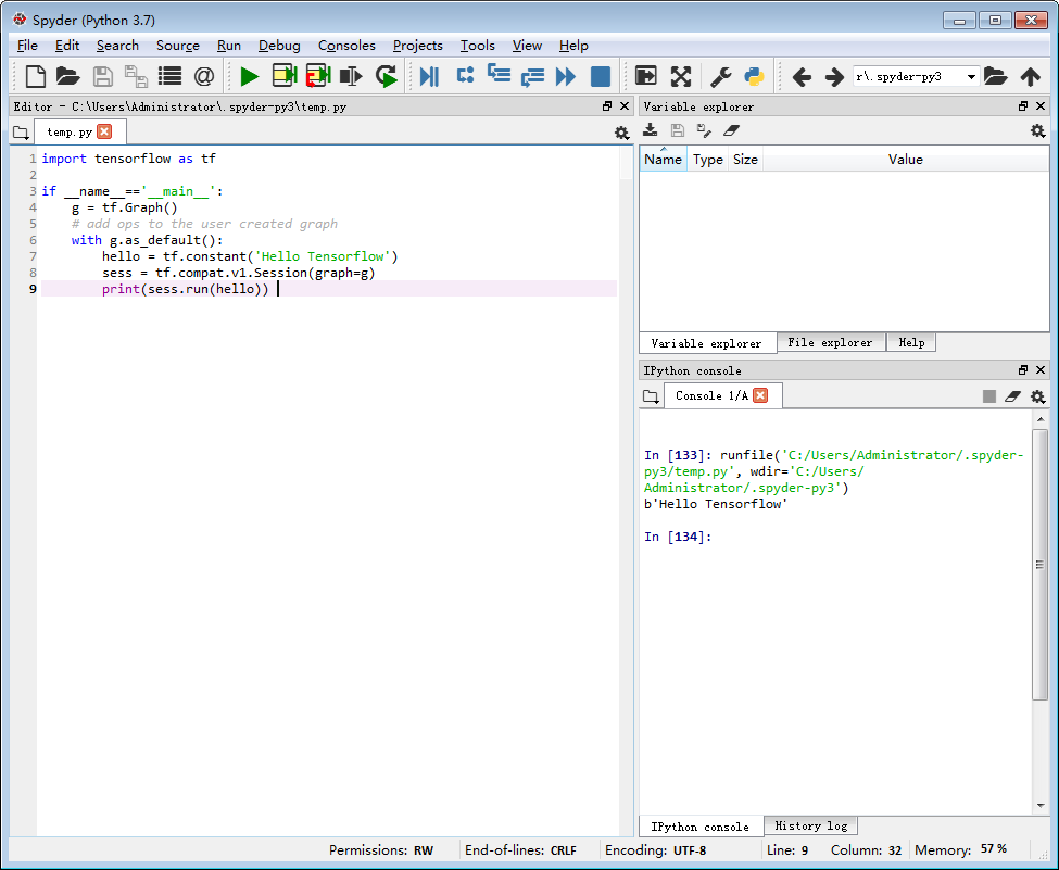
说明：python3.7.4 ，tensorflow2.0 

 若对您有用，请赞助个棒棒糖~

SSD-Tensorflow： 3 步运行 TensorFlow 单图片多盒目标检测器

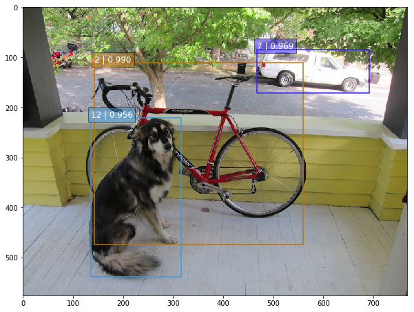
昨天类似的 YOLO： https://www.v2ex.com/t/392671#reply0

下载这个项目

https://github.com/balancap/SSD-Tensorflow

解压 checkpoint files in ./checkpoint

unzip ssd_300_vgg.ckpt.zip

运行 jupyter 文件命令

jupyter notebook notebooks/ssd_notebook.ipynb

项目说明： http://www.tensorflownews.com/2017/09/22/ssd-single-shot-multibox-detector-in-tensorflow/

项目地址： https://github.com/balancap/SSD-Tensorflow

更多 TensorFlow 教程： http://www.tensorflownews.com

关于Tensorflow精度为.99，但预测很糟糕和tensorflow准确率的问题我们已经讲解完毕，感谢您的阅读，如果还想了解更多关于Centos6安装TensorFlow及TensorFlowOnSpark、github/tensorflow/tensorflow/contrib/slim/、hello tensorflow，我的第一个tensorflow程序、SSD-Tensorflow： 3 步运行 TensorFlow 单图片多盒目标检测器等相关内容，可以在本站寻找。