此处将为大家介绍关于Seaborn配置隐藏默认的matplotlib的详细内容,并且为您解答有关matplotlib隐藏边框的相关问题,此外,我们还将为您介绍关于Jupyterlab/Notebook
此处将为大家介绍关于Seaborn配置隐藏默认的matplotlib的详细内容,并且为您解答有关matplotlib隐藏边框的相关问题,此外,我们还将为您介绍关于Jupyterlab / Notebook 中的交互式 matplotlib 图(使用 ipympl 的 %matplotlib 小部件)仅工作一次然后消失、Matplotlib AttributeError:模块'matplotlib.cbook'没有属性'_define_aliases'、Matplotlib Superscript format in matplotlib plot legend 上标下标、Matplotlib Toolkits:python 高级绘图库 seaborn的有用信息。
本文目录一览:- Seaborn配置隐藏默认的matplotlib(matplotlib隐藏边框)
- Jupyterlab / Notebook 中的交互式 matplotlib 图(使用 ipympl 的 %matplotlib 小部件)仅工作一次然后消失
- Matplotlib AttributeError:模块'matplotlib.cbook'没有属性'_define_aliases'
- Matplotlib Superscript format in matplotlib plot legend 上标下标
- Matplotlib Toolkits:python 高级绘图库 seaborn
")
Seaborn配置隐藏默认的matplotlib(matplotlib隐藏边框)
Seaborn提供了一些图形,这些图形对于科学数据表示非常有趣。因此,我开始使用这些Seaborn图形以及其他自定义的matplotlib图。问题是一旦我这样做:
import seaborn as sb此导入似乎为全局设置了seaborn的图形参数,然后该导入下方的所有matplotlib图形都获得了seaborn参数(它们具有灰色背景,linewithd更改等)。
在SO中有一个答案解释了如何使用matplotlib配置生成海图,但是我想要的是在同时使用两个库时保持matplotlib配置参数不变,并能够在需要时生成原始海图。
答案1
小编典典从seaborn版本0.8(2017年7月)开始,图形样式在导入时不再更改:
导入seaborn时,不再应用默认的[seaborn]样式。现在有必要显式调用
set()或一个或多个set_style()
,set_context()和set_palette()。相应地,该seaborn.apionly模块已被弃用。
您可以使用来选择任何情节的样式plt.style.use()。
import matplotlib.pyplot as pltimport seaborn as snsplt.style.use(''seaborn'') # switch to seaborn style# plot code# ...plt.style.use(''default'') # switches back to matplotlib style# plot code# ...# to see all available stylesprint(plt.style.available)了解更多有关plt.style()。
仅工作一次然后消失")
Jupyterlab / Notebook 中的交互式 matplotlib 图(使用 ipympl 的 %matplotlib 小部件)仅工作一次然后消失
如何解决Jupyterlab / Notebook 中的交互式 matplotlib 图(使用 ipympl 的 %matplotlib 小部件)仅工作一次然后消失?
我再次尝试在 Jupyter Notebooks 中为我的学生使用交互式 matplotlib 图。我的计划是使用 JupyterLab,因为普通的 Notebook 界面在学生中不太受欢迎。这是一个两芯 MWE 笔记本:
import numpy as np
%matplotlib widget
import matplotlib.pyplot as plt
下一个单元格:
plt.figure(1)
x = np.arange(100)
y = x*x
plt.plot(x,y)
plt.show()
当我运行这些单元格时,我确实得到了一个交互式 Matplotlib 图。但是当我第二次运行第二个单元格时,绘图窗口消失而没有警告或错误,只有在我在第二个单元格之前重新运行第一个单元格时才会返回。经典笔记本界面显示相同的行为,删除 plt.show() 或 plt.figure() 也没有区别。
我在 venv 环境中的 Windows 10 计算机上本地运行 Jupyter 服务器,安装了以下版本:
Python           : 3.8.2
ipympl           : 0.7.0

jupyter core     : 4.7.1
jupyter-notebook : 6.3.0
qtconsole        : not installed
ipython          : 7.23.1
ipykernel        : 5.5.4
jupyter client   : 6.1.12
jupyter lab      : 3.0.14
nbconvert        : 6.0.7
ipywidgets       : 7.6.3
nbformat         : 5.1.3
traitlets        : 5.0.5
在我的非专业人士看来,启动期间的消息似乎没问题:
[I 2021-05-12 10:10:48.065 LabApp] JupyterLab extension loaded from d:\envs\pyfda_38\lib\site-packages\jupyterlab
[I 2021-05-12 10:10:48.065 LabApp] JupyterLab application directory is D:\envs\pyfda_38\share\jupyter\lab
[I 2021-05-12 10:10:48.069 ServerApp] jupyterlab | extension was successfully loaded.
[I 2021-05-12 10:10:48.488 ServerApp] nbclassic | extension was successfully loaded.
[I 2021-05-12 10:10:48.489 ServerApp] Serving notebooks from local directory: D:\Daten\xxx
[I 2021-05-12 10:10:48.489 ServerApp] Jupyter Server 1.6.4 is running at:
[I 2021-05-12 10:10:48.489 ServerApp] http://localhost:8888/lab?token=xxxx
我得到的唯一(可能)相关警告是
[W 2021-05-12 10:10:55.256 LabApp] Could not determine jupyterlab build status without nodejs
是我做错了什么,还是 ipympl 的交互图还不够成熟,无法进行 BYOD 课程?
解决方法
它在每次通过将魔术命令移动到第二个单元格来激活 matplotlib 交互式支持时起作用:
%matplotlib widget
plt.figure(1)
x = np.arange(100)
y = x*x
plt.plot(x,y)
plt.show()

Matplotlib AttributeError:模块'matplotlib.cbook'没有属性'_define_aliases'
如何解决Matplotlib AttributeError:模块''matplotlib.cbook''没有属性''_define_aliases''?
我有这个确切的错误。问题是matplotlib的2个软件包分别是conda和pip所安装的2个软件包
要对此进行测试:
$ conda list matplotlib
matplotlib 2.0.2 np113py35_0 matplotlib 2.1.1
问题!固定:
$ pip uninstall matplotlib
强制将matplotlib升级到想要的pip版本的好主意:
$ conda install matplotlib=2.1.1
解决方法
当尝试使用pyplot在jupyter上绘制图形时,我正在运行以下代码:
import matplotlib.pyplot as plt
plt.plot([1,2,3,4])
plt.ylabel(''some numbers'')
plt.show()
这将返回以下错误:
AttributeError                            Traceback (most recent call last)
<ipython-input-16-51b004b519a9> in <module>()
----> 1 get_ipython().run_line_magic(''matplotlib'',''inline'')
      2
      3
      4 import matplotlib.pyplot as plt
      5 plt.plot([1,4])

c:\program files (x86)\microsoft visual studio\shared\python36_64\lib\site-packages\IPython\core\interactiveshell.py in run_line_magic(self,magic_name,line,_stack_depth)
   2129                 kwargs[''local_ns''] = sys._getframe(stack_depth).f_locals
   2130             with self.builtin_trap:
-> 2131                 result = fn(*args,**kwargs)
   2132             return result
   2133

<decorator-gen-108> in matplotlib(self,line)

c:\program files (x86)\microsoft visual studio\shared\python36_64\lib\site-packages\IPython\core\magic.py in <lambda>(f,*a,**k)
    185     # but it''s overkill for just that one bit of state.
    186     def magic_deco(arg):
--> 187         call = lambda f,**k: f(*a,**k)
    188
    189         if callable(arg):

c:\program files (x86)\microsoft visual studio\shared\python36_64\lib\site-packages\IPython\core\magics\pylab.py in matplotlib(self,line)
     97             print("Available matplotlib backends: %s" % backends_list)
     98         else:
---> 99             gui,backend = self.shell.enable_matplotlib(args.gui)
    100             self._show_matplotlib_backend(args.gui,backend)
    101

c:\program files (x86)\microsoft visual studio\shared\python36_64\lib\site-packages\IPython\core\interactiveshell.py in enable_matplotlib(self,gui)
   3049                 gui,backend = pt.find_gui_and_backend(self.pylab_gui_select)
   3050
-> 3051         pt.activate_matplotlib(backend)
   3052         pt.configure_inline_support(self,backend)
   3053

c:\program files (x86)\microsoft visual studio\shared\python36_64\lib\site-packages\IPython\core\pylabtools.py in activate_matplotlib(backend)
    308     matplotlib.rcParams[''backend''] = backend
    309
--> 310     import matplotlib.pyplot
    311     matplotlib.pyplot.switch_backend(backend)
    312

c:\program files (x86)\microsoft visual studio\shared\python36_64\lib\site-packages\matplotlib\pyplot.py in <module>()
     30 from cycler import cycler
     31 import matplotlib
---> 32 import matplotlib.colorbar
     33 import matplotlib.image
     34 from matplotlib import rcsetup,style

c:\program files (x86)\microsoft visual studio\shared\python36_64\lib\site-packages\matplotlib\colorbar.py in <module>()
     28 import matplotlib.artist as martist
     29 import matplotlib.cbook as cbook
---> 30 import matplotlib.collections as collections
     31 import matplotlib.colors as colors
     32 import matplotlib.contour as contour

c:\program files (x86)\microsoft visual studio\shared\python36_64\lib\site-packages\matplotlib\collections.py in <module>()
     17
     18 import matplotlib as mpl
---> 19 from . import (_path,artist,cbook,cm,colors as mcolors,docstring,20                lines as mlines,path as mpath,transforms)
     21

c:\program files (x86)\microsoft visual studio\shared\python36_64\lib\site-packages\matplotlib\lines.py in <module>()
    206
    207
--> 208 @cbook._define_aliases({
    209     "antialiased": ["aa"],210     "color": ["c"],AttributeError: module ''matplotlib.cbook'' has no attribute ''_define_aliases''
没有jupyter,我的matplotlib一直运行良好。从那时起,我再次尝试完全重新安装matplotlib,jupyter和python,但仍然收到相同的错误。也许有人遇到过同样的问题?

Matplotlib Superscript format in matplotlib plot legend 上标下标
在绘图的标题、坐标轴的文字中用上标或下标
格式:$正常文字^上标$
import matplotlib.pyplot as plt

fig, ax = plt.subplots()
ax.set(title=r'This is an expression $e^{\sin(\omega\phi)}$',
       xlabel='meters $10^1$', ylabel=r'Hertz $(\frac{1}{s})$')
plt.show()

import matplotlib.pyplot as plt
import numpy as np
from scipy.optimize import curve_fit

x_data = np.linspace(0.05,1,101)
y_data = 1/x_data
noise = np.random.normal(0, 1, y_data.shape)
y_data2 = y_data + noise

def func_power(x, a, b):
    return a*x**b

popt, pcov= curve_fit(func_power, x_data, y_data2)

plt.figure()
plt.scatter(x_data, y_data2, label = 'data')
plt.plot(x_data, popt[0] * x_data ** popt[1], label = ("$y = {{{}}}x^{{{}}}$").format(round(popt[0],2), round(popt[1],2)))
plt.plot(x_data, x_data**3, label = '$x^3$')
plt.legend()
plt.show()

import matplotlib.pyplot as plt
import numpy as np
from scipy.optimize import curve_fit

x_data = np.linspace(0.05,1,101)
y_data = 1/x_data
noise = np.random.normal(0, 1, y_data.shape)
y_data2 = y_data + noise

def func_power(x, a, b):
    return a*x**b

popt, pcov= curve_fit(func_power, x_data, y_data2)

plt.figure(figsize=(4, 3))
plt.title('Losses')
plt.ylabel('Loss')
plt.xlabel('Epoch')
plt.scatter(x_data, y_data2, label = 'data')
plt.plot(x_data, popt[0] * x_data ** popt[1], label = ("$y = {{{}}}x^{{{}}}$").format(round(popt[0],2), round(popt[1],2)))
plt.plot(x_data, x_data**3, label = '$x^3$')
plt.legend()
plt.show()
REF
https://stackoverflow.com/questions/53781815/superscript-format-in-matplotlib-plot-legend
https://stackoverflow.com/questions/21226868/superscript-in-python-plots

Matplotlib Toolkits:python 高级绘图库 seaborn
http://blog.csdn.net/pipisorry/article/details/49515745
Seaborn 介绍
seaborn
(Not distributed with matplotlib)
seaborn is a highlevel interface for drawing statistical graphics with matplotlib. Itaims to make visualization a central part of exploring andunderstanding complex datasets.
[seaborn ¶]Matplotlib 是 Python 主要的绘图库。但是不建议你直接使用它,原因与不推荐你使用 NumPy 是一样的。虽然 Matplotlib 很强大,它本身就很复杂,你的图经过大量的调整才能变精致。因此,作为替代推荐一开始使用 Seaborn。
Seaborn 本质上使用 Matplotlib 作为核心库(就像 Pandas 对 NumPy 一样)。
seaborn 的优点:
- 默认情况下就能创建赏心悦目的图表。(只有一点,默认不是 jet colormap)
- 创建具有统计意义的图
- 能理解 pandas 的 DataFrame 类型,所以它们一起可以很好地工作。
安装 pip install seaborn
Note: lz 发现,就算你不用 seaborn 绘图,只要在 matplotlib 绘图中加上 seaborn 的 import 语句,就会以 seaborn 的图形方式展示图片,具有 seaborn 的效果。如:
import seaborn
import matplotlib.pyplot as plt
注意要显示出图形,需要引入 matplotlib 并 plt.show () 出来。
皮皮 blog
Seaborn 使用
Style functions: API | Tutorial
Color palettes: API | Tutorial
Distribution plots: API | Tutorial
Regression plots: API | Tutorial
Categorical plots: API | Tutorial
Axis grid objects: API | Tutorial
分布图绘制 Distribution plots
jointplot(x, y[, data, kind, stat_func, ...]) |
Draw a plot of two variables with bivariate and univariate graphs. |
pairplot(data[, hue, hue_order, palette, ...]) |
Plot pairwise relationships in a dataset. |
distplot(a[, bins, hist, kde, rug, fit, ...]) |
Flexibly plot a univariate distribution of observations. |
kdeplot(data[, data2, shade, vertical, ...]) |
Fit and plot a univariate or bivariate kernel density estimate. |
rugplot(a[, height, axis, ax]) |
Plot datapoints in an array as sticks on an axis. |
单变量绘制 distplot
seaborn.distplot(a, bins=None, hist=True, kde=True, rug=False, fit=None, hist_kws=None, kde_kws=None, rug_kws=None, fit_kws=None, color=None, vertical=False, norm_hist=False, axlabel=None, label=None, ax=None)
Note:
1 如果想显示统计个数而不是概率,需要同时设置 norm_hist=False, kde=False。
2 自己指定 fit 的函数 from scipy import stats ... fit=stats.norm
>>> import seaborn as sns, numpy as np
>>> sns.set(rc={"figure.figsize": (8, 4)}); np.random.seed(0)
>>> x = np.random.randn(100)
>>> ax = sns.distplot(x)
双变量 + 单变量统一绘制 jointplot
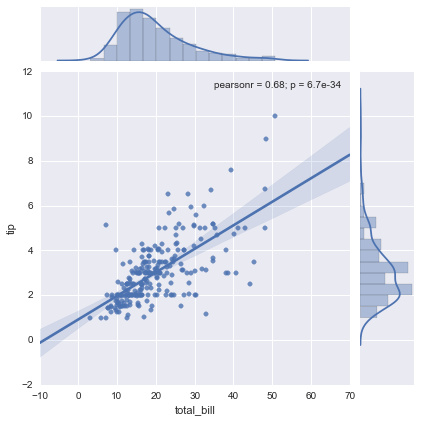
使用 matplotlib 重新绘制这幅图的话需要相当多的(丑陋)代码,包括调用 scipy 执行线性回归并手动利用线性回归方程绘制直线(我甚至想不出怎么在边界绘图,怎么计算置信区间)。
[ the tutorial on quantitative linear models]
与 Pandas 的 DataFrame 很好地工作
数据有自己的结构。通常我们感兴趣的包含不同的组或类(这种情况下使用 pandas 中 groupby 的功能会让人感到很神奇)。比如 tips(小费)的数据集是这样的:
Out[9]:
| total_bill | tip | sex | smoker | day | time | size | |
|---|---|---|---|---|---|---|---|
| 0 | 16.99 | 1.01 | Female | No | Sun | Dinner | 2 |
| 1 | 10.34 | 1.66 | Male | No | Sun | Dinner | 3 |
| 2 | 21.01 | 3.50 | Male | No | Sun | Dinner | 3 |
| 3 | 23.68 | 3.31 | Male | No | Sun | Dinner | 2 |
| 4 | 24.59 | 3.61 | Female | No | Sun | Dinner | 4 |
我们可能想知道吸烟者给的小费是否与不吸烟的人不同。没有 seaborn 的话,这需要使用 pandas 的 groupby 功能,并通过复杂的代码绘制线性回归直线。使用 seaborn 的话,我们可以给 col 参数提供列名,按我们的需要划分数据:
回归图绘制 Regression plots
lmplot(x, y, data[, hue, col, row, palette, ...]) |
Plot data and regression model fits across a FacetGrid. |
regplot(x, y[, data, x_estimator, x_bins, ...]) |
Plot data and a linear regression model fit. |
residplot(x, y[, data, lowess, x_partial, ...]) |
Plot the residuals of a linear regression. |
interactplot(x1, x2, y[, data, filled, ...]) |
Visualize a continuous two-way interaction with a contour plot. |
coefplot(formula, data[, groupby, ...]) |
Plot the coefficients from a linear model. |
sns . lmplot ( "total_bill" , "tip" , tips , col = "smoker" ) ;
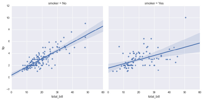
很整洁吧?随着你研究得越深,你可能想更细粒度地控制这些图表的细节。因为 seaborn 只是调用了 matplotlib,那时你可能会想学习这个库。
from: http://blog.csdn.net/pipisorry/article/details/49515745ref: [seaborn API reference]*
[Seaborn tutorial]*
Python 和数据科学的起步指南
Example gallery
Python 数据可视化模块:Seaborn
关于Seaborn配置隐藏默认的matplotlib和matplotlib隐藏边框的介绍现已完结,谢谢您的耐心阅读,如果想了解更多关于Jupyterlab / Notebook 中的交互式 matplotlib 图(使用 ipympl 的 %matplotlib 小部件)仅工作一次然后消失、Matplotlib AttributeError:模块'matplotlib.cbook'没有属性'_define_aliases'、Matplotlib Superscript format in matplotlib plot legend 上标下标、Matplotlib Toolkits:python 高级绘图库 seaborn的相关知识,请在本站寻找。
本文标签:


