本文将带您了解关于gprof,Valgrindandgperftools-anevaluationofsometoolsforapplicationlevelCPUprofilingon的新内容，另外

本文将带您了解关于gprof, Valgrind and gperftools - an evaluation of some tools for application level CPU profiling on的新内容，另外，我们还将为您提供关于Allocation Profiling in Java Mission Control、Amazon Personalize can now use 10X more item attributes to improve relevance of recommendations、An Empirical Evaluation of Generic Convolutional and Recurrent Networks for Sequence Modeling、android – GATT over SPP profile for bluetooth communication？的实用信息。

本文目录一览：

• gprof, Valgrind and gperftools - an evaluation of some tools for application level CPU profiling on
• Allocation Profiling in Java Mission Control
• Amazon Personalize can now use 10X more item attributes to improve relevance of recommendations
• An Empirical Evaluation of Generic Convolutional and Recurrent Networks for Sequence Modeling
• android – GATT over SPP profile for bluetooth communication？

gprof, Valgrind and gperftools - an evaluation of some tools for application level CPU profiling on

In this post I give an overview of my evaluation of three different CPU profiling tools: gperftools, Valgrind and gprof. I evaluated the three tools on usage, functionality, accuracy and runtime overhead.

The usage of the different profilers is demonstrated with the small demo program cpuload, available via my github repository gklingler/cpuProfilingDemo. The intent of cpuload.cpp is just to generate some CPU load - it does nothing useful. The bash scripts in the same repo (which are also listed below) show how to compile/link the cpuload.cpp appropriately and execute the resulting executable to get the CPU profiling data.

gprof

The GNU profiler gprof uses a hybrid approach of compiler assisted instrumentation and sampling. Instrumentation is used to gather function call information (e.g. to be able to generate call graphs and count the number of function calls). To gather profiling information at runtime, a sampling process is used. This means, that the program counter is probed at regular intervals by interrupting the program with operating system interrupts. As sampling is a statistical process, the resulting profiling data is not exact but are rather a statistical approximation gprof statistical inaccuracy.

Creating a CPU profile of your application with gprof requires the following steps:

1. compile and link the program with a compatible compiler and profiling enabled (e.g. gcc -pg).
2. execute your program to generate the profiling data file (default filename: gmon.out)
3. run gprof to analyze the profiling data

Let’s apply this to our demo application:

#!/bin/bash

# build the program with profiling support (-gp)
g++ -std=c++11 -pg cpuload.cpp -o cpuload

# run the program; generates the profiling data file (gmon.out)
./cpuload

# print the callgraph
gprof cpuload

The gprof output consists of two parts: the flat profile and the call graph.

The flat profile reports the total execution time spent in each function and its percentage of the total running time. Function call counts are also reported. Output is sorted by percentage, with hot spots at the top of the list.

Gprof’s call graph is a textual call graph representation which shows the caller and callees of each function.

For detailed information on how to interpret the callgraph, take a look at the official documentation. You can also generate a graphical representation of the callgraph with gprof2dot - a tool to generate a graphical representation of the gprof callgraph)).

The overhead (mainly caused by instrumentation) can be quite high: estimated to 30-260%1 2.

gprof does not support profiling multi-threaded applications and also cannot profile shared libraries. Even if there exist workarounds to get threading support3, the fact that it cannot profile calls into shared libraries, makes it totally unsuitable for today’s real-world projects.

valgrind/callgrind

Valgrind4 is an instrumentation framework for building dynamic analysis tools. Valgrind is basically a virtual machine with just in time recompilation of x86 machine code to some simpler RISC-like intermediate code: UCode. It does not execute x86 machine code directly but it “simulates” the on the fly generated UCode. There are various Valgrind based tools for debugging and profiling purposes. Depending on the chosen tool, the UCode is instrumented appropriately to record the data of interest. For performance profiling, we are interested in the tool callgrind: a profiling tool that records the function call history as a call-graph.

For analyzing the collected profiling data, there is is the amazing visualization tool KCachegrind5. It represents the collected data in a very nice way what tremendously helps to get an overview about whats going on.

Creating a CPU profile of your application with valgrind/callgrind is really simple and requires the following steps:

1. compile your program with debugging symbols enabled (to get a meaningful call-graph)
2. execute your program with valgrind --tool=callgrind ./yourprogram to generate the profiling data file
3. analyze your profiling data with e.g. KCachegrind

Let’s apply this our demo application (profile_valgrind.sh):

#!/bin/bash

# build the program (no special flags are needed)
g++ -std=c++11 cpuload.cpp -o cpuload

# run the program with callgrind; generates a file callgrind.out.12345 that can be viewed with kcachegrind
valgrind --tool=callgrind ./cpuload

# open profile.callgrind with kcachegrind
kcachegrind profile.callgrind

In contrast to gprof, we don’t need to rebuild our application with any special compile flags. We can execute any executable as it is with valgrind. Of course the executed program should contain debugging information to get an expressive call graph with human readable symbol names.

Below you see a KCachegrind with the profiling data of our cpuload demo:

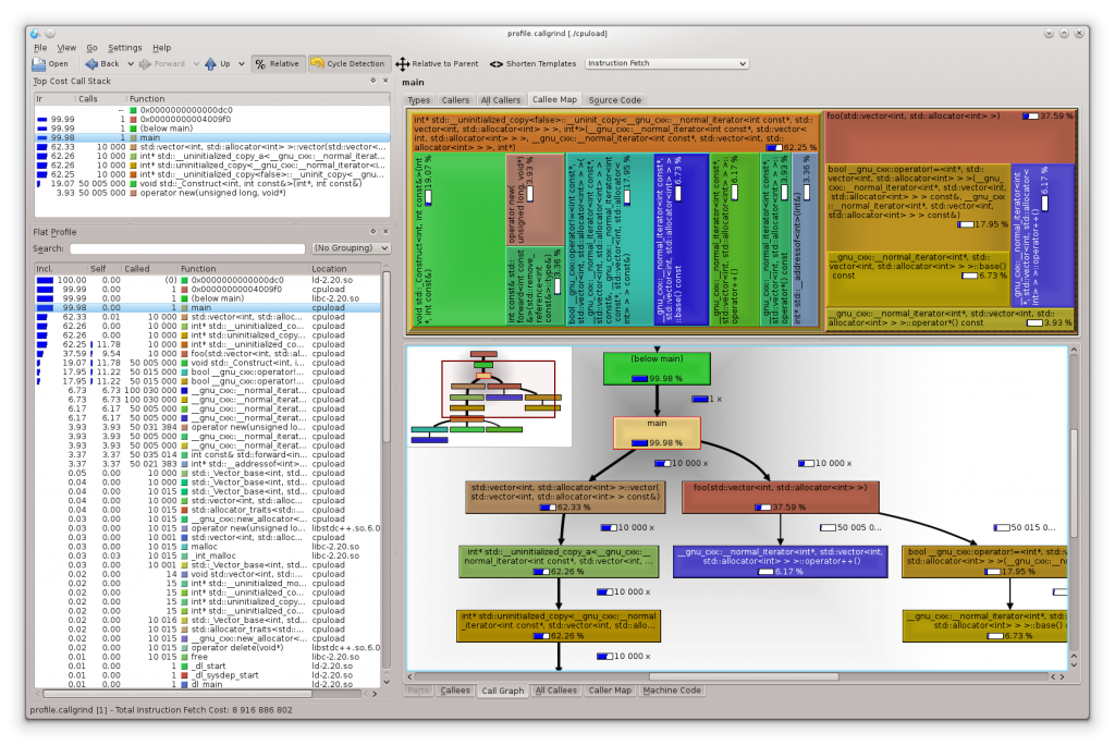
A downside of Valgrind is the enormous slowdown of the profiled application (around a factor of 50x) what makes it impracticable to use for larger/longer running applications. The profiling result itself is not influenced by the measurement.

gperftools

Gperftools from Google provides a set of tools aimed for analyzing and improving performance of multi-threaded applications. They offer a CPU profiler, a fast thread aware malloc implementation, a memory leak detector and a heap profiler. We focus on their sampling based CPU profiler.

Creating a CPU profile of selected parts of your application with gperftools requires the following steps:

1. compile your program with debugging symbols enabled (to get a meaningful call graph) and link gperftools profiler.so
2. #include <gperftools/profiler.h> and surround the sections you want to profile with ProfilerStart("nameOfProfile.log"); and ProfilerStop();
3. execute your program to generate the profiling data file(s)
4. To analyze the profiling data, use pprof (distributed with gperftools) or convert it to a callgrind compatible format and analyze it with KCachegrind

Let’s apply this our demo application (profile_gperftools.sh):

#!/bin/bash

# build the program; For our demo program, we specify -DWITHGPERFTOOLS to enable the gperftools specific #ifdefs
g++ -std=c++11 -DWITHGPERFTOOLS -lprofiler -g ../cpuload.cpp -o cpuload

# run the program; generates the profiling data file (profile.log in our example)
./cpuload

# convert profile.log to callgrind compatible format
pprof --callgrind ./cpuload profile.log > profile.callgrind

# open profile.callgrind with kcachegrind
kcachegrind profile.callgrind

Alternatively, profiling the whole application can be done without any changes or recompilation/linking, but I will not cover this here as this is not the recommended approach. But you can find more about this in the docs.

The gperftools profiler can profile multi-threaded applications. The run time overhead while profiling is very low and the applications run at “native speed”. We can again use KCachegrind for analyzing the profiling data after converting it to a cachegrind compatible format. I also like the possibility to be able to selectively profile just certain areas of the code, and if you want to, you can easily extend your program to enable/disable profiling at runtime.

Conclusion and comparison

gprof is the dinosaur among the evaluated profilers - its roots go back into the 1980’s. It seems it was widely used and a good solution during the past decades. But its limited support for multi-threaded applications, the inability to profile shared libraries and the need for recompilation with compatible compilers and special flags that produce a considerable runtime overhead, make it unsuitable for using it in today’s real-world projects.

Valgrind delivers the most accurate results and is well suited for multi-threaded applications. It’s very easy to use and there is KCachegrind for visualization/analysis of the profiling data, but the slow execution of the application under test disqualifies it for larger, longer running applications.

The gperftools CPU profiler has a very little runtime overhead, provides some nice features like selectively profiling certain areas of interest and has no problem with multi-threaded applications. KCachegrind can be used to analyze the profiling data. Like all sampling based profilers, it suffers statistical inaccuracy and therefore the results are not as accurate as with Valgrind, but practically that’s usually not a big problem (you can always increase the sampling frequency if you need more accurate results). I’m using this profiler on a large code-base and from my personal experience I can definitely recommend using it.

I hope you liked this post and as always, if you have questions or any kind of feedback please leave a comment below.

1. GNU gprof Profiler ↑
2. Low-Overhead Call Path Profiling of Unmodified, Optimized Code for higher order object oriented programs, Yu Kai Hong, Department of Mathematics at National Taiwan University; July 19, 2008, ACM 1-59593-167/8/06/2005 ↑
3. workaround to use gprof with multithreaded applications ↑
4. Valgrind ↑
5. KCachegrind ↑

Allocation Profiling in Java Mission Control

Allocation Profiling in Java Mission Control

Thursday, September 12, 2013  - By Marcus

With the Hotspot JDK 7u40 there is a nifty new tool called Java Mission Control. Users of the nifty old tool JRockit Mission Control will recognize a lot of the features. This particular blog entry focuses on how to do allocation profiling with the Java Flight Recorder.

The JVM is a wonderful little piece of virtualization technology that gives you the illusion of an infinite heap. However that comes at a cost. Sometimes the JVM will need to find out exactly what on your heap is in use, and throw the rest away – a so called garbage collection. This is because the physical memory available to the JVM indeed is limited, and memory will have to be reclaimed and reused when it is no longer needed. In timing sensitive applications, such as trading systems and telco applications, such pauses can be quite costly. There are various tuning that can be done for the GC to make it less likely to occur. But I digress. One way to garbage collect less, is of course to allocate less.

Sometimes you may want to find out where the allocation pressure is caused by your application. There are various reasons as to why you may have reached this conclusion. The most common one is probably that the JVM is having to garbage collect more often and/or longer than you think is reasonable.

The JFR Allocation Event

In the Java Flight Recorder implementation in HotSpot 7u40 there are two allocation events that can assist in finding out where the allocations are taking place in your application: the Allocation in new TLAB and the Allocation outside TLAB events.

Just like for most events provided with the HotSpot JDK, there is of course a custom user interface for analyzing this in Mission Control, but before going there I thought we’d take a moment to discuss the actual events.

First you need to make sure they are recorded. If you bring up the default (continuous) template, you will notice that allocation profiling is off by default. Either turn it on, or use the profiling template. The reason it is off by default is that it may produce quite a lot of events, and it is a bit hard to estimate the overhead since it will vary a lot with the particular allocation behaviour of your application.

The Log tab in the Events tab group is an excellent place to look at individual events. Let’s check out what these actually contain:

They contain the allocation size of whatever was allocated, the stack trace for what caused the allocation, the class of what was allocated, and time information. In the case of the inside TLAB allocation events, they also contain the size of the TLAB.

Note that we, in the case of the (inside) TLAB allocation events, are not emitting an event for each and every location – that would be way too expensive. We are instead creating an event for the first allocation in a new TLAB. This means that we get a sampling of sorts of the thread local allocations taking place.

Also, note that in JRockit we used to have TLA events that perfectly corresponded to the allocations done in the nursery, and large object allocation events that corresponded to allocation done directly in old space. This is a little bit more complicated in HotSpot. The outside TLAB allocation events can both correspond to allocations done due to an allocation causing a young collection, and the subsequent allocation of the object in the Eden as well as the direct allocation of a humongous object directly in old space. In other words, don’t worry too much if you see the allocation of a few small objects among the outside of TLAB events. Normally these would be very few though, so in practice the distinction is probably not that important.

Using the Allocations Tab

The allocations tab actually consists of three sub tabs:

1. General

2. Allocation in new TLAB

3. Allocation outside TLAB

The General tab provides an overview and some statistics of the available events, such as total memory allocated for the two different event types. Depending on what your overarching goal is (e.g. tuning TLAB size, reducing overall allocation) you may use this information differently. In the example below it would seem prudent to focus on the inside TLAB allocations, as they contribute way more to the total allocation pressure.

The Allocation in new TLAB tab provides three more types of visualization specific to the in new TLAB events: Allocation by Class, Allocation by Thread and Allocation Profile. The Allocation Profile is simply the aggregated stack trace tree for all of the events. In the example below it can be seen that Integer object allocations correspond to almost all the allocations in the system. Selecting the Integer class in the histogram table shows the aggregated stack traces for all the Integer allocations, and in this example all of them originate from the same place, as seen below (click in pictures to show them in full size).

The Allocation outside TLAB tab works exactly the same way as the Allocation in new TLAB tab, only this time it is, of course, for the Allocation outside TLAB events:

Limitations

Since the Allocation in new TLAB events only represents a sample of the total thread local allocations, having only one event will say very little about the actual distribution. The more events, the more accurate the picture. Also, if the allocation behaviour vary wildly during the recording, it may be hard to establish a representative picture of the thread local allocations.

Thanks to Nikita Salnikov for requesting this blog entry! 

Further reading and useful links

Related Blogs:    
Java Mission Control Finally Released    
Creating Flight Recordings    
My JavaOne 2013 Sessions    
Low Overhead Method Profiling with Mission Control

The Mission Control home page:    
http://oracle.com/missioncontrol

Mission Control Base update site for Eclipse:    
http://download.oracle.com/technology/products/missioncontrol/updatesites/base/5.2.0/eclipse/

Mission Control Experimental update site (Mission Control plug-ins):    
http://download.oracle.com/technology/products/missioncontrol/updatesites/experimental/5.2.0/eclipse/

The Mission Control Facebook Community Page (not kidding):    
http://www.facebook.com/pages/Java-Mission-Control/275169442493206

Amazon Personalize can now use 10X more item attributes to improve relevance of recommendations

https://amazonaws-china.com/blogs/machine-learning/amazon-personalize-can-now-use-10x-more-item-attributes-to-improve-relevance-of-recommendations/

Amazon Personalize is a machine learning service which enables you to personalize your website, app, ads, emails, and more, with custom machine learning models which can be created in Amazon Personalize, with no prior machine learning experience. AWS is pleased to announce that Amazon Personalize now supports ten times more item attributes for modeling in Personalize. Previously, you could use up to five item attributes while building an ML model in Amazon Personalize. This limit is now 50 attributes. You can now use more information about your items, for example, category, brand, price, duration, size, author, year of release etc., to increase the relevance of recommendations.

In this post, you learn how to add item metadata with custom attributes to Amazon Personalize and create a model using this data and user interactions. This post uses the Amazon customer reviews data for beauty products. For more information and to download this data, see Amazon Customer Reviews Dataset. We will use the history of what items the users have reviewed along with user and item metadata to generate product recommendations for them.

Pre-processing the data

To model the data in Amazon Personalize, you need to break it into the following datasets:

• Users – Contains metadata about the users
• Items – Contains metadata about the items
• Interactions – Contains interactions (for this post, reviews) and metadata about the interactions

For each respective dataset, this post uses the following attributes:

• Users – customer_id, helpful_votes, and total_votes
• Items – product_id, product_category, and product_parent
• Interactions – product_id, customer_id, review_date, and star_rating

This post does not use the other attributes available, which include marketplace, review_id, product_title, vine, verified_purchase, review_headline, and review_body.

Additionally, to conform with the keywords in Amazon Personalize, this post renames customer_id to USER_ID, product_id to ITEM_ID, and review_date to TIMESTAMP.

To download and process the data for input to Amazon Personalize, use the following Python example codes.

For the Users dataset, enter the following code:

#Downloading data
$aws s3 cp s3://amazon-reviews-pds/tsv/amazon_reviews_us_Beauty_v1_00.tsv.gz .
$gunzip amazon_reviews_us_Beauty_v1_00.tsv.gz

#Generating the user dataset
import pandas as pd
fields = [''customer_id'', ''helpful_votes'', ''total_votes'']
df = pd.read_csv(''amazon_reviews_us_Beauty_v1_00.tsv'', sep=''\t'', usecols=fields)
df = df.rename(columns={''customer_id'':''USER_ID''})
df.to_csv(''User_dataset.csv'', index = None, header=True)

The following screenshot shows the Users dataset. This output can be generated by

df.head()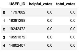

For the Items dataset, enter the following code:

#Generating the item dataset
fields = [''product_id'', ''product_category'', ''product_parent'']
df1 = pd.read_csv(''amazon_reviews_us_Beauty_v1_00.tsv'', sep=''\t'', usecols=fields)
df1= df1.rename(columns={''product_id'':''ITEM_ID''})

#Clip category names to 999 characters to confirm to Personalize limits
maxlen = 999
for index, row in df1.iterrows():
    product_category = row[''product_category''][:maxlen]
df1.to_csv(''Item_dataset.csv'', index = None, header=True)

The following screenshot shows the Items dataset. This output can be generated by

df1.head()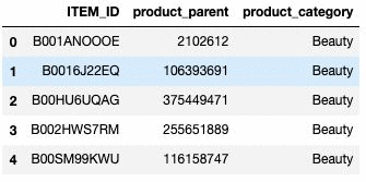

For the Interactions dataset, enter the following code:

#Generating the interactions dataset
from datetime import datetime
fields = [''product_id'', ''customer_id'', ''review_date'', ''star_rating'']
df2 = pd.read_csv(''amazon_reviews_us_Beauty_v1_00.tsv'', sep=''\t'', usecols=fields, low_memory=False)
df2= df2.rename(columns={''product_id'':''ITEM_ID'', ''customer_id'':''USER_ID'', ''review_date'':''TIMESTAMP''})

#Converting timstamp to UNIX timestamp and rounding milliseconds
num_errors =0
for index, row in df2.iterrows(): 
    time_input= row["TIMESTAMP"]
    try:
        time_input = datetime.strptime(time_input, "%Y-%m-%d")
        timestamp = round(datetime.timestamp(time_input))
        df2.set_value(index, "TIMESTAMP", timestamp)
    except:
        print("exception at index: {}".format(index))
        num_errors += 1
print("Total rows in error: {}".format(num_errors))
df2.to_csv("Interaction_dataset.csv", index = None, header=True)

The following screenshot shows the Interactions dataset. This output can be generated by

df2.head()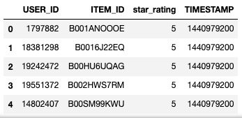

Ingesting the data

After you process the preceding data, you can ingest it in Amazon Personalize.

Creating a dataset group

To create a dataset group to store events (user interactions) sent by your application and the metadata for users and items, complete the following steps:

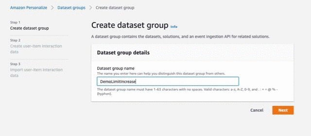
1. On the Amazon Personalize console, under Dataset groups, choose Create dataset group.
2. For Dataset group name, enter the name of your dataset group. This post enters the name DemoLimitIncrease.
3. Choose Next.
   
   

Creating a dataset and defining schema

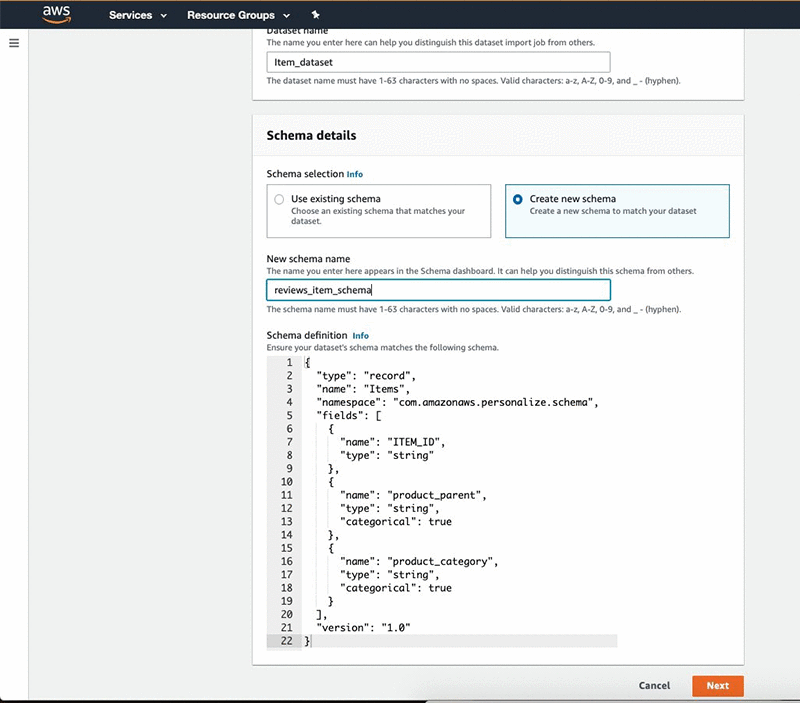
After you create the dataset group, create a dataset and define schema for each of them. The following steps are for your Items dataset:

1. For Dataset name, enter a name.
2. Under Schema details, select Create new schema.
3. For New schema name, enter a name.
4. For Schema definition, enter the following code:

   {
   	"type": "record",
   	"name": "Items",
   	"namespace": "com.amazonaws.personalize.schema",
   	"fields": [
   		{
   			"name": "ITEM_ID",
   			"type": "string"
   		},
   		{
   			"name": "product_parent",
   			"type": "string",
   			"categorical": true
   		},
   		{
   			"name": "product_category",
   			"type": "string",
   			"categorical": true
   		}
   	],
   	"version": "1.0"}

5. Choose Next.
   
   

Follow the same steps for the Users and Interactions datasets and define the schema to conform to the columns you want to import.

Importing the data

After you create the dataset, import the data from Amazon S3. Make sure you provide Amazon Personalize read access to your bucket. To import your Items data, complete the following steps:

1. Under Dataset import job details, for Dataset import job name, enter a name.
2. For IAM Service role, choose AmazonPersonalize-ExecutionRole.
3. For Data location, enter the location of your S3 bucket.
4. Choose Create dataset import job.
   
   

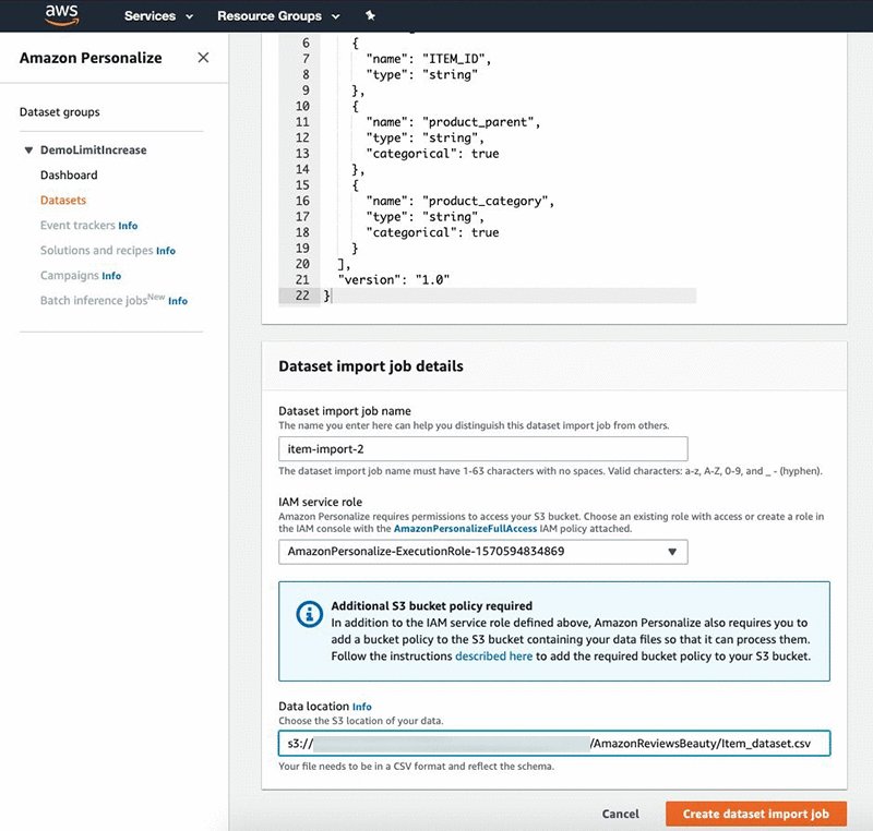
Follow the same steps to import your Users and Interactions datasets.

Training a model

After you ingest the data into Amazon Personalize, you are ready to train a model (solutionVersion). To do so, map the recipe (algorithm) you want to use to your use case. The following are your available options:

• For user personalization, such as recommending items to a user, use one of the following recipes:
  • HRNN – Trains only on interaction data and provides a baseline
  • HRNN-Metadata – Trains on interaction+user, item, and interaction metadata and is recommended when you have such data available
  • HRNN-Coldstart – Use when you want to recommend cold (new) items to a user
• For recommending items similar to an input item, use SIMS.
• For reranking a list of input items for a given user, use Personalized-Ranking.

This post uses the HRNN-Metadata recipe to define a solution and then train a solutionVersion (model). Complete the following steps:

1. On the Amazon Personalize console, under Dataset groups, choose DemoLimitIncrease.
2. Choose Solutions.
3. Choose Create solution.
4. Under Solution configuration, for Solution name, enter a name
5. For Recipe selection, select Manual.
6. For Recipe, choose aws-hrnn-metadata.
7. Choose Next.
   
   

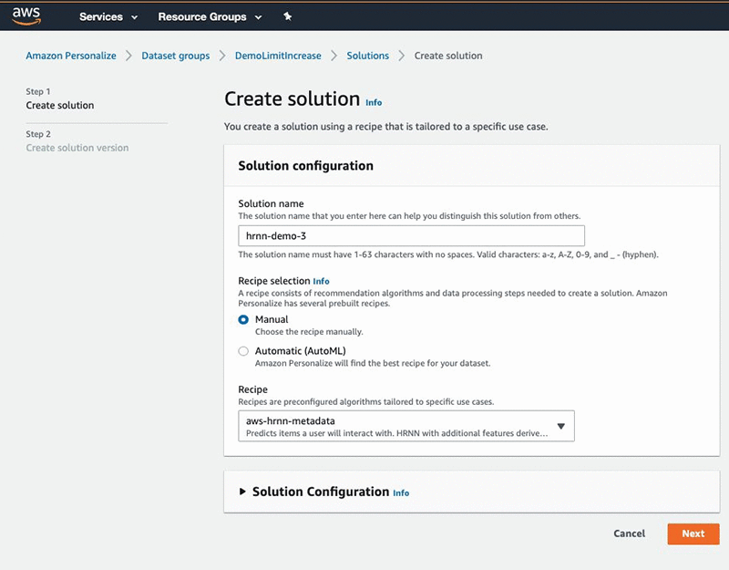
You can also change the default hyperparameters or perform hyperparameter optimization for a solution.

Getting recommendations

To get recommendations, create a campaign using the solution and solution version you just created. Complete the following steps:

1. Under Dataset groups, under DemoLimitIncrease, choose Campaigns.
2. Choose Create new campaign.
3. Under Campaign details, for Campaign name, enter a name
4. For Solution, choose the solution name from previous step.
5. For Solution version ID, choose the solution version you just created.
6. For Minimum provisioned transactions per second, enter 1.
7. Choose Create campaign.
   
   
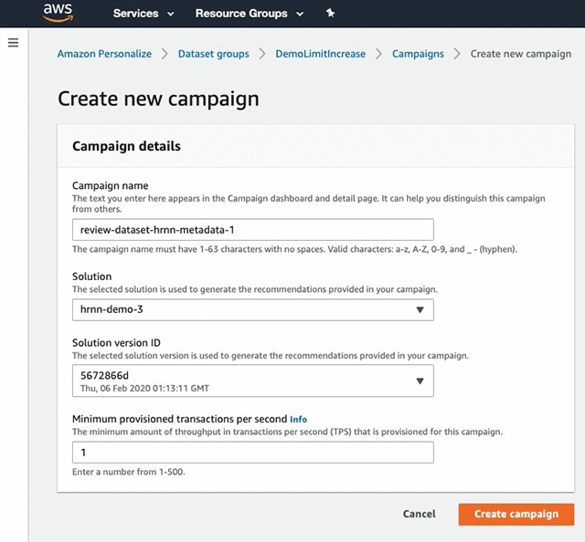
8. After the campaign is created you can see the details in the console and use it to get recommendations.
   
   

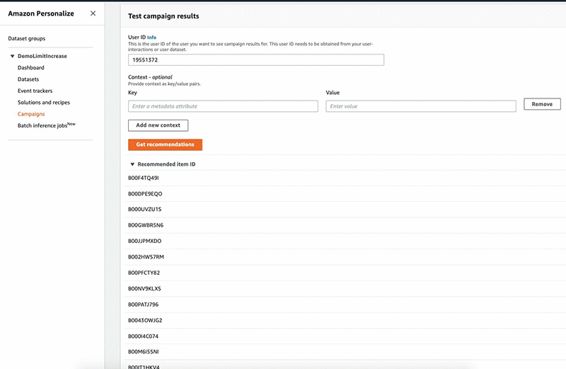
After you set up the campaign, you can programmatically call the campaign to get recommendations in form of item IDs. You can also use the console to get the recommendations and perform spot checks. Additionally, Amazon Personalize offers the ability to batch process recommendations. For more information, see Now available: Batch Recommendations in Amazon Personalize.

Conclusion

You can now use these recommendations to power display experiences, such as personalize the homepage of your beauty website based on what you know about the user or send a promotional email with recommendations. Performing real-time recommendations with Amazon Personalize requires you to also send user events as they occur. For more information, see Amazon Personalize is Now Generally Available. Get started with Amazon Personalize today!

---

About the author

Vaibhav Sethi is the Product Manager for Amazon Personalize. He focuses on delivering products that make it easier to build machine learning solutions. In his spare time, he enjoys hiking and reading.

 

 

 

 

 

An Empirical Evaluation of Generic Convolutional and Recurrent Networks for Sequence Modeling

An Empirical Evaluation of Generic Convolutional and Recurrent Networks for Sequence Modeling 
Original time: 2018-05-16 16:09:15

Updated on 2019-09-27 10:26:42

 

 

Paper: https://arxiv.org/pdf/1803.01271.pdf 

Code：http://github.com/locuslab/TCN

 

1. Background and Motivation：

一提到时序建模，大部分人第一反应是 RNN, LSTM；而最近有些工作表明，CNN 在某些时序任务上也取得了顶尖的实验效果。那么，问题来了，这个序列 CNN 模型，是只对某些特定的任务有效，还是对很多任务都可以建模呢？本着这个动机，作者进行了充分的实验，并且结合最新的一些 CNN 方面的技巧，重新设计了 sequential CNN 模型，提出了 TCN， 网络结构，用卷积的方式进行序列数据的处理，并且取得了和更加复杂的 RNN、LSTM、GRU 等模型相当的精度。作者在文中提到：sequence modeling 和 recurrent networks 之间的常规联系，应该被重新认识。TCN 的网络结构不但比 LSTM GRU 等取得了更好的效果，并且结构也更加简单，明了。对于后续的序列建模问题，可能是一个新的起点。

 

Temporal Convolutional Networks : 

　　TCNs 的特点有：

　　1). the convolutions in the architecture are casual, meaning that there is no information "leakage" from future to past; 

　　2). the architecture can take  a sequence of any length and map it to an output sequence of the same length, just as with an RNN. 

　　3). we emphasize how to build very long effective history size using a combination of very deep networks and dilated convolutions. 

 

　　1. Sequence Modeling :

　　输入是一个序列，如：x₀, ... , x_T；对应输出的 label 是 y₀, ... , y_T。而序列模型就是要学习这么一个映射函数，从输入到输出，即：

　　

　　但是，这种方法以 autoregressive prediction 为核心，但是，不能直接捕获下面的 domain：machine translation, or sequence to sequence prediction，因为：在这些情况下，整个的输入可以被用来预测每一个输出（since in these cases the entire input sentence can be used to predict each output）。

　　2. Casual Convlutions : 

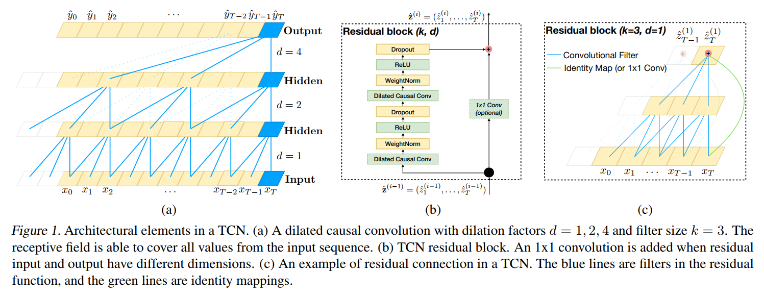
　　TCNs 是基于两个原则的：

　　（1）the fact that the network produces an output of the same length as the input（输入和输出保持一致）, 

　　（2）the fact that there can be no leakage from the future into the past（从未来到过去，没做信息泄露）. 

　　

　　为了满足第一点，TCNs 采用全卷积网络结构。每一个 hidden layer 和 input layer 是相同的，and zero padding of length (kernel size -1) is added to keep subsequent layers the same length as previous ones. 

　　为了满足第二点，TCNs 采用 casual convolutions, where an output at time t is convolved only with elements from time t and earlier in the previous layer. 

　　那么，TCNs 就是：TCN = 1D FCN + casual convolutions. 

　　

　　这种基本的设计方法的主要不足之处在于：为了得到一个较长的历史尺寸，我们需要一个非常深的网络 或者 非常大的 filters。

　　3. Dilated Convolutions : 

　　为了使得 filter size 尽可能大，我们采用 dilated convolutions，that enable an exponentially large receptive field. 

　　正式的，对于 1-D sequence input x , 以及 a filter f , 空洞卷积操作 F 在输入序列中元素 s 可以定义为：

　　

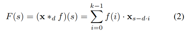
　　其中，d 是空洞系数，k 是filter size，s-di accounts for the direction of the past. 

　　Using larger dilation enables an output at the top level to represent a wider range of inputs, thus effectively expanding the receptive field of a ConvNet. 

　　这给我们增加 TCN 的感受野，提供了两个思路：

　　(1). choosing larger filter sizes k ; 

　　(2). increasing the dilation factor d, where the effective history of one such layer is (k-1)d. 

　　4. Residual Connnections : 

　　此处的残差连接，就是借鉴了何凯明的 residual network，即：将之前的信息和转换后的信息，都作为当前的输入，从而使得网络层数非常深的时候，仍然能够得到不错的效果：

　　

　　This effectively allows layers to learn modifications to the identity mapping rather than the entire transformation, which has repeatly been shown to benefit very deep networks. 

　　

　　5. Discussion : 

　　本小结总结了 TCN 用于 sequence modeling 的几个优势和劣势：

　　（1）Parallelilsm　　RNN 的预测总是需要上一个时刻完毕后，才可以进行。但是 CNN 的则没有这个约束，因为 the same filter is used in each layer. 

　　（2）Flexible receptive field size　　TCN 可以在不同的 layer 采用不同的 receptive field size。

　　（3）Stable gradients　　不同于 RNN 结构，TCN has a backpropagation path different from the temporal direction of the sequence. 所以 TCN 就没有 RNN 结构中梯度消失或者梯度爆炸的情况。

　　（4）Low memory requirement for training　　LSTM or GRU 由于需要存储很多 cell gates 的信息，所以需要很大的内存，但是由于 filter 是共享的，内存的利用仅仅依赖于网络的深度。而作者也发现：gated RNNs likely to use up to a multiplicative factor more memory than TCNs. 

　　（5）Variable length inputs 　　TCNs can also take in inputs of arbitrary length by sliding the 1D convolutional kernels. 

 

　　两个明显的劣势在于：

　　（1）Data storage during evalution.  

　　（2）Potential parameter change for a transfer of domain. 

 

 

android – GATT over SPP profile for bluetooth communication？

我们今天的关于gprof, Valgrind and gperftools - an evaluation of some tools for application level CPU profiling on的分享就到这里，谢谢您的阅读，如果想了解更多关于Allocation Profiling in Java Mission Control、Amazon Personalize can now use 10X more item attributes to improve relevance of recommendations、An Empirical Evaluation of Generic Convolutional and Recurrent Networks for Sequence Modeling、android – GATT over SPP profile for bluetooth communication？的相关信息，可以在本站进行搜索。

本文标签：

• gprof
• Valgrind
• gperftools
• CPU_profiling