以上就是给各位分享hashCodemethodperformancetuning,同时本文还将给你拓展(转)EnsembleMethodsforDeepLearningNeuralNetworksto
以上就是给各位分享hashCode method performance tuning,同时本文还将给你拓展(转) Ensemble Methods for Deep Learning Neural Networks to Reduce Variance and Improve Performance、.NET Core 性能分析: xUnit.Performance 简介、A DB2 Performance Tuning Roadmap、A DB2 Performance Tuning Roadmap --DIVE INTO LOCK等相关知识,如果能碰巧解决你现在面临的问题,别忘了关注本站,现在开始吧!
本文目录一览:- hashCode method performance tuning
- (转) Ensemble Methods for Deep Learning Neural Networks to Reduce Variance and Improve Performance
- .NET Core 性能分析: xUnit.Performance 简介
- A DB2 Performance Tuning Roadmap
- A DB2 Performance Tuning Roadmap --DIVE INTO LOCK

hashCode method performance tuning
hashCode method performance tuning
by Mikhail Vorontsov
In this chapter we will discuss various implications of hashCode method implementation on application performance.
The main purpose of hashCode method is to allow an object to be a key in the hash map or a member of a hash set. In this case an object should also implement equals(Object) method, which is consistent with hashCode implementation:
- If a.equals(b) then a.hashCode() == b.hashCode()
- If hashCode() was called twice on the same object, it should return the same result provided that the object was not changed
hashCode from performance point of view
From the performance point of view, the main objective for your hashCode method implementation is to minimize the number of objects sharing the same hash code. All JDK hash based collections store their values in an array. Hash code is used to calculate an initial lookup position in this array. After that equals is used to compare given value with values stored in the internal array. So, if all values have distinct hash codes, this will minimize the possibility of hash collisions. On the other hand, if all values will have the same hash code, hash map (or set) will degrade into a list with operations on it having O(n2) complexity.
For more details, read about collision resolution in hash maps. JDK is using a method calledopen addressing, but there is another method called “chaining” – all key-value pairs with the same hash code are stored in a linked list.
Let’s see the difference in hash code quality. We will compare a normal String with a string wrapper, which overrides hashCode method in order to return the same hash code for all objects.
1
2
3
4
5
6
7
8
9
10
11
12
13
14
15
16
17
18
19
20
21
private static class SlowString { public final String m_str; public SlowString( final String str ) { this.m_str = str; } @Override public int hashCode() { return 37; } @Override public boolean equals(Object o) { if (this == o) return true; if (o == null || getClass() != o.getClass()) return false; final SlowString that = ( SlowString ) o; return !(m_str != null ? !m_str.equals(that.m_str) : that.m_str != null); } }
Here is a testing method. It worth quoting because we will use it again later. It accepts a prepared list of objects (in order not to include these objects creation time in our test) and calls Map.put followed by Map.containsKey on each value in the list.
1
2
3
4
5
6
7
8
9
10
11
12
13
14
private static void testMapSpeed( final List lst, final String name ) { final Map<Object, Object> map = new HashMap<Object, Object>( lst.size() ); int cnt = 0; final long start = System.currentTimeMillis(); for ( final Object obj : lst ) { map.put( obj, obj ); if ( map.containsKey( obj ) ) ++cnt; } final long time = System.currentTimeMillis() - start; System.out.println( "Time for " + name + " is " + time / 1000.0 + " sec, cnt = " + cnt ); }
Both String and SlowString objects are created in a loop as "ABCD" + i. It took 0.041 sec to process 100,000 String objects. As for the same number of SlowString objects, it took 82.5 seconds to process them.
As it turned out, String class has exceptional quality hashCode method. Let’s write another test. We will create a list of Strings. First half of them will be equal to "ABCdef*&" + i, second half – "ABCdef*&" + i + "ghi" (to ensure that changes in the middle of the string with a constant tail will not decrease hash code quality). We will create 1M, 5M, 10M and 20M strings and see how many of them will share hash codes and how many strings will share the same hash code. This is test output:
Number of duplicate hashCodes for 1000000 strings = 0

Number of duplicate hashCodes for 5000000 strings = 196
Number of hashCode duplicates = 2 count = 196

Number of duplicate hashCodes for 10000000 strings = 1914
Number of hashCode duplicates = 2 count = 1914

Number of duplicate hashCodes for 20000000 strings = 17103
Number of hashCode duplicates = 2 count = 17103
So, as you can see, only a very small number of strings is sharing the same hash code and it is very unlikely that one hash code will be shared by more than two strings (unless they are specially crafted, of course). Of course, your data may be different – just run a similar test on your typical keys.
Autogenerated hashCode for long fields
It is worth mentioning how hashCode method is generated for long datatype by most of IDEs. Here is a generated hashCode method for a class with 2 long fields:
1
2
3
4
5
public int hashCode() { int result = (int) (val1 ^ (val1 >>> 32)); result = 31 * result + (int) (val2 ^ (val2 >>> 32)); return result; }
And here is the similar method generated for a class with 2 int fields:
1
2
3
4
5
public int hashCode() { int result = val1; result = 31 * result + val2; return result; }
As you see, long is treated differently. Similar code is used in java.util.Arrays.hashCode(long a[]). Actually, you will get better hash code distribution if you will extract high and low 32 bits of long and treat them as int while calculating a hash code. Here is an improvedhashCode method for a class with 2 long fields (note that this method runs slower than an original method, but quality of new hash codes will allow hash collections to run faster even at the expense of hashCode slowdown).
1
2
3
4
5
6
public int hashCode() { int result = (int) val1; result = 31 * result + (int) (val1 >>> 32); result = 31 * result + (int) val2; return 31 * result + (int) (val2 >>> 32); }
Here are results of testMapSpeed method for processing 10M objects of all three kinds. They were initialized with the same values (all longs actually fit into int values).
As you can see, hashCode update makes a difference. Not so big, but worth noticing for performance critical code.
Use case: How to benefit from String.hashCode quality
Let’s assume we have a map from string identifiers to some values. Map keys (string identifiers) are not stored anywhere else in memory (at most only some of them may be stored somewhere else at a time). We have already collected all map entries, for example, on the first pass of some two phase algorithm. On the second phase we will need to query map values by keys. We will query our map only using existing map keys.
How can we improve the map? As you have seen before, String.hashCode returns mostly distinct values. We can scan all keys, calculate hash codes of all keys and find not unique hash codes:
1 2 3 4 5 6 7 8 9 10 11 12 13 14 15 16 17 18Map<Integer, Integer> cnt = new HashMap<Integer, Integer>( max ); for ( final String s : dict.keySet() ) { final int hash = s.hashCode(); final Integer count = cnt.get( hash ); if ( count != null ) cnt.put( hash, count + 1 ); else cnt.put( hash, 1 ); } //keep only not unique hash codes final Map<Integer, Integer> mult = new HashMap<Integer, Integer>( 100 ); for ( final Map.Entry<Integer, Integer> entry : cnt.entrySet() ) { if ( entry.getValue() > 1 ) mult.put( entry.getKey(), entry.getValue() ); }
Now we can create 2 maps out of the old one. Let’s assume for simplicity that old map values were just Objects. In this case, we will end up with Map<Integer, Object> and Map<String, Object> (for production code Trove TIntObjectHashMap is recommended instead ofMap<Integer, Object>). First map will contain mapping from unique hash codes to values, second map – mapping from strings with not unique hash codes to values.
1
2
3
4
5
6
7
8
9
10
11
12
final Map<Integer, Object> unique = new HashMap<Integer, Object>( 1000 ); final Map<String, Object> not_unique = new HashMap<String, Object>( 1000 ); //dict - original map for ( final Map.Entry<String, Object> entry : dict.entrySet() ) { final int hashCode = entry.getKey().hashCode(); if ( mult.containsKey( hashCode ) ) not_unique.put( entry.getKey(), entry.getValue() ); else unique.put( hashCode, entry.getValue() ); }
Now, in order to get a value, we need to query unique map first and not_unique map if first query has not returned a valid result:
1
2
3
4
5
6
7
8
public Object get( final String key ) { final int hashCode = key.hashCode(); Object value = m_unique.get( hashCode ); if ( value == null ) value = m_not_unique.get( key ); return value; }
In some rare cases you may still have too many (by your opinion) string keys in thenon_unique map. In this case first of all try replacing hash code calculation with eitherjava.util.zip.CRC32 or java.util.zip.Adler32 calculation (Adler32 is faster than CRC32, but has a bit worse distribution). As a last resort, try combining 2 independent functions in onelong key: lower 32 bits for one function, higher 32 bits for another. The choice of hash functions is obvious: Object.hashCode, java.util.zip.CRC32 or java.util.zip.Adler32.
How to compress a set even better than a map
Previous use case discussed how to get rid of keys in a map. Actually, we may achieve even better results for sets. I can see 2 cases when sets may be used: first is splitting an original set into several subsets and querying if an identifier belongs to a given subset; second is writing a spellchecker – you will query your set with any unforeseeable values (that’s the nature of spellcheckers), but some mistakes are not critical (if another word has the same hash code as your allegedly unique hash code, you could report such word as correct). In both cases sets will be extremely useful for us.
If we will just apply previous logic to sets, we will end up with Set<Integer> for unique hash codes and Set<String> for non-unique ones. We can optimize at least a couple of things here.
If we will limit range of values generated by hashCode method to some limited number (2^20 if fine, for example), then we can replace a Set<Integer> with a BitSet, as it was discussed inBit sets article. We can always select sufficient limit for hash code if we know size of our original set in advance (before compression).
The next objective is to check how many identifiers with non-unique has codes you still have. Improve your hashCode method or increase a range of allowed hash code values if you have too many of non-unique hash codes. In the perfect case all your identifiers will have unique hash codes (it is not too difficult to achieve, by the way). As a result, you will be able to useBitSets instead of large sets of strings.
See also
A new hashing method was added to String class in Java 1.7.0_06. For more details seeChanges to String internal representation made in Java 1.7.0_06 article.
Summary
Try to improve distribution of results of your hashCode method. This is far more important than to optimize that method speed. Never write a hashCode method which returns a constant.
String.hashCode results distribution is nearly perfect, so you can sometimes substituteStrings with their hash codes. If you are working with sets of strings, try to end up withBitSets, as described in this article. Performance of your code will greatly improve.
Post navigation
← java.util.zip.CRC32 and java.util.zip.Adler32 performance Changes to String internal representation made in Java 1.7.0_06 →SUMMARY
Java performance tuning guide summary - all you could read on this website in one page.
GOOGLE ADS
MOST POPULAR
- Changes to String internal representation made in Java 1.7.0_06
- Using double/long vs BigDecimal for monetary calculations
- Trove library: using primitive collections for performance
- java.util.ArrayList performance guide
- Performance of various methods of binary serialization in Java
- Various types of memory allocation in Java
- Java collections overview
GOOGLE ADS
TAGS
hashCode method performance tuning
by Mikhail Vorontsov
In this chapter we will discuss various implications of hashCode method implementation on application performance.
The main purpose of hashCode method is to allow an object to be a key in the hash map or a member of a hash set. In this case an object should also implement equals(Object) method, which is consistent with hashCode implementation:
- If a.equals(b) then a.hashCode() == b.hashCode()
- If hashCode() was called twice on the same object, it should return the same result provided that the object was not changed
hashCode from performance point of view
From the performance point of view, the main objective for your hashCode method implementation is to minimize the number of objects sharing the same hash code. All JDK hash based collections store their values in an array. Hash code is used to calculate an initial lookup position in this array. After that equals is used to compare given value with values stored in the internal array. So, if all values have distinct hash codes, this will minimize the possibility of hash collisions. On the other hand, if all values will have the same hash code, hash map (or set) will degrade into a list with operations on it having O(n2) complexity.
For more details, read about collision resolution in hash maps. JDK is using a method calledopen addressing, but there is another method called “chaining” – all key-value pairs with the same hash code are stored in a linked list.
Let’s see the difference in hash code quality. We will compare a normal String with a string wrapper, which overrides hashCode method in order to return the same hash code for all objects.
1
2
3
4
5
6
7
8
9
10
11
12
13
14
15
16
17
18
19
20
21
private static class SlowString { public final String m_str; public SlowString( final String str ) { this.m_str = str; } @Override public int hashCode() { return 37; } @Override public boolean equals(Object o) { if (this == o) return true; if (o == null || getClass() != o.getClass()) return false; final SlowString that = ( SlowString ) o; return !(m_str != null ? !m_str.equals(that.m_str) : that.m_str != null); } }
Here is a testing method. It worth quoting because we will use it again later. It accepts a prepared list of objects (in order not to include these objects creation time in our test) and calls Map.put followed by Map.containsKey on each value in the list.
1
2
3
4
5
6
7
8
9
10
11
12
13
14
private static void testMapSpeed( final List lst, final String name ) { final Map<Object, Object> map = new HashMap<Object, Object>( lst.size() ); int cnt = 0; final long start = System.currentTimeMillis(); for ( final Object obj : lst ) { map.put( obj, obj ); if ( map.containsKey( obj ) ) ++cnt; } final long time = System.currentTimeMillis() - start; System.out.println( "Time for " + name + " is " + time / 1000.0 + " sec, cnt = " + cnt ); }
Both String and SlowString objects are created in a loop as "ABCD" + i. It took 0.041 sec to process 100,000 String objects. As for the same number of SlowString objects, it took 82.5 seconds to process them.
As it turned out, String class has exceptional quality hashCode method. Let’s write another test. We will create a list of Strings. First half of them will be equal to "ABCdef*&" + i, second half – "ABCdef*&" + i + "ghi" (to ensure that changes in the middle of the string with a constant tail will not decrease hash code quality). We will create 1M, 5M, 10M and 20M strings and see how many of them will share hash codes and how many strings will share the same hash code. This is test output:
Number of duplicate hashCodes for 1000000 strings = 0

Number of duplicate hashCodes for 5000000 strings = 196
Number of hashCode duplicates = 2 count = 196

Number of duplicate hashCodes for 10000000 strings = 1914
Number of hashCode duplicates = 2 count = 1914

Number of duplicate hashCodes for 20000000 strings = 17103
Number of hashCode duplicates = 2 count = 17103
So, as you can see, only a very small number of strings is sharing the same hash code and it is very unlikely that one hash code will be shared by more than two strings (unless they are specially crafted, of course). Of course, your data may be different – just run a similar test on your typical keys.
Autogenerated hashCode for long fields
It is worth mentioning how hashCode method is generated for long datatype by most of IDEs. Here is a generated hashCode method for a class with 2 long fields:
1
2
3
4
5
public int hashCode() { int result = (int) (val1 ^ (val1 >>> 32)); result = 31 * result + (int) (val2 ^ (val2 >>> 32)); return result; }
And here is the similar method generated for a class with 2 int fields:
1
2
3
4
5
public int hashCode() { int result = val1; result = 31 * result + val2; return result; }
As you see, long is treated differently. Similar code is used in java.util.Arrays.hashCode(long a[]). Actually, you will get better hash code distribution if you will extract high and low 32 bits of long and treat them as int while calculating a hash code. Here is an improvedhashCode method for a class with 2 long fields (note that this method runs slower than an original method, but quality of new hash codes will allow hash collections to run faster even at the expense of hashCode slowdown).
1
2
3
4
5
6
public int hashCode() { int result = (int) val1; result = 31 * result + (int) (val1 >>> 32); result = 31 * result + (int) val2; return 31 * result + (int) (val2 >>> 32); }
Here are results of testMapSpeed method for processing 10M objects of all three kinds. They were initialized with the same values (all longs actually fit into int values).
As you can see, hashCode update makes a difference. Not so big, but worth noticing for performance critical code.
Use case: How to benefit from String.hashCode quality
Let’s assume we have a map from string identifiers to some values. Map keys (string identifiers) are not stored anywhere else in memory (at most only some of them may be stored somewhere else at a time). We have already collected all map entries, for example, on the first pass of some two phase algorithm. On the second phase we will need to query map values by keys. We will query our map only using existing map keys.
How can we improve the map? As you have seen before, String.hashCode returns mostly distinct values. We can scan all keys, calculate hash codes of all keys and find not unique hash codes:
1 2 3 4 5 6 7 8 9 10 11 12 13 14 15 16 17 18Map<Integer, Integer> cnt = new HashMap<Integer, Integer>( max ); for ( final String s : dict.keySet() ) { final int hash = s.hashCode(); final Integer count = cnt.get( hash ); if ( count != null ) cnt.put( hash, count + 1 ); else cnt.put( hash, 1 ); } //keep only not unique hash codes final Map<Integer, Integer> mult = new HashMap<Integer, Integer>( 100 ); for ( final Map.Entry<Integer, Integer> entry : cnt.entrySet() ) { if ( entry.getValue() > 1 ) mult.put( entry.getKey(), entry.getValue() ); }
Now we can create 2 maps out of the old one. Let’s assume for simplicity that old map values were just Objects. In this case, we will end up with Map<Integer, Object> and Map<String, Object> (for production code Trove TIntObjectHashMap is recommended instead ofMap<Integer, Object>). First map will contain mapping from unique hash codes to values, second map – mapping from strings with not unique hash codes to values.
1
2
3
4
5
6
7
8
9
10
11
12
final Map<Integer, Object> unique = new HashMap<Integer, Object>( 1000 ); final Map<String, Object> not_unique = new HashMap<String, Object>( 1000 ); //dict - original map for ( final Map.Entry<String, Object> entry : dict.entrySet() ) { final int hashCode = entry.getKey().hashCode(); if ( mult.containsKey( hashCode ) ) not_unique.put( entry.getKey(), entry.getValue() ); else unique.put( hashCode, entry.getValue() ); }
Now, in order to get a value, we need to query unique map first and not_unique map if first query has not returned a valid result:
1
2
3
4
5
6
7
8
public Object get( final String key ) { final int hashCode = key.hashCode(); Object value = m_unique.get( hashCode ); if ( value == null ) value = m_not_unique.get( key ); return value; }
In some rare cases you may still have too many (by your opinion) string keys in thenon_unique map. In this case first of all try replacing hash code calculation with eitherjava.util.zip.CRC32 or java.util.zip.Adler32 calculation (Adler32 is faster than CRC32, but has a bit worse distribution). As a last resort, try combining 2 independent functions in onelong key: lower 32 bits for one function, higher 32 bits for another. The choice of hash functions is obvious: Object.hashCode, java.util.zip.CRC32 or java.util.zip.Adler32.
How to compress a set even better than a map
Previous use case discussed how to get rid of keys in a map. Actually, we may achieve even better results for sets. I can see 2 cases when sets may be used: first is splitting an original set into several subsets and querying if an identifier belongs to a given subset; second is writing a spellchecker – you will query your set with any unforeseeable values (that’s the nature of spellcheckers), but some mistakes are not critical (if another word has the same hash code as your allegedly unique hash code, you could report such word as correct). In both cases sets will be extremely useful for us.
If we will just apply previous logic to sets, we will end up with Set<Integer> for unique hash codes and Set<String> for non-unique ones. We can optimize at least a couple of things here.
If we will limit range of values generated by hashCode method to some limited number (2^20 if fine, for example), then we can replace a Set<Integer> with a BitSet, as it was discussed inBit sets article. We can always select sufficient limit for hash code if we know size of our original set in advance (before compression).
The next objective is to check how many identifiers with non-unique has codes you still have. Improve your hashCode method or increase a range of allowed hash code values if you have too many of non-unique hash codes. In the perfect case all your identifiers will have unique hash codes (it is not too difficult to achieve, by the way). As a result, you will be able to useBitSets instead of large sets of strings.
See also
A new hashing method was added to String class in Java 1.7.0_06. For more details seeChanges to String internal representation made in Java 1.7.0_06 article.
Summary
Try to improve distribution of results of your hashCode method. This is far more important than to optimize that method speed. Never write a hashCode method which returns a constant.
String.hashCode results distribution is nearly perfect, so you can sometimes substituteStrings with their hash codes. If you are working with sets of strings, try to end up withBitSets, as described in this article. Performance of your code will greatly improve.
 Ensemble Methods for Deep Learning Neural Networks to Reduce Variance and Improve Performance")
(转) Ensemble Methods for Deep Learning Neural Networks to Reduce Variance and Improve Performance
Ensemble Methods for Deep Learning Neural Networks to Reduce Variance and Improve Performance
2018-12-19 13:02:45
This blog is copied from: https://machinelearningmastery.com/ensemble-methods-for-deep-learning-neural-networks/
Deep learning neural networks are nonlinear methods.
They offer increased flexibility and can scale in proportion to the amount of training data available. A downside of this flexibility is that they learn via a stochastic training algorithm which means that they are sensitive to the specifics of the training data and may find a different set of weights each time they are trained, which in turn produce different predictions.
Generally, this is referred to as neural networks having a high variance and it can be frustrating when trying to develop a final model to use for making predictions.
A successful approach to reducing the variance of neural network models is to train multiple models instead of a single model and to combine the predictions from these models. This is called ensemble learning and not only reduces the variance of predictions but also can result in predictions that are better than any single model.
In this post, you will discover methods for deep learning neural networks to reduce variance and improve prediction performance.
After reading this post, you will know:
- Neural network models are nonlinear and have a high variance, which can be frustrating when preparing a final model for making predictions.
- Ensemble learning combines the predictions from multiple neural network models to reduce the variance of predictions and reduce generalization error.
- Techniques for ensemble learning can be grouped by the element that is varied, such as training data, the model, and how predictions are combined.
Let’s get started.

Ensemble Methods to Reduce Variance and Improve Performance of Deep Learning Neural Networks
Photo by University of San Francisco’s Performing Arts, some rights reserved.
Overview
This tutorial is divided into four parts; they are:
- High Variance of Neural Network Models
- Reduce Variance Using an Ensemble of Models
- How to Ensemble Neural Network Models
- Summary of Ensemble Techniques
High Variance of Neural Network Models
Training deep neural networks can be very computationally expensive.
Very deep networks trained on millions of examples may take days, weeks, and sometimes months to train.
Google’s baseline model […] was a deep convolutional neural network […] that had been trained for about six months using asynchronous stochastic gradient descent on a large number of cores.
— Distilling the Knowledge in a Neural Network, 2015.
After the investment of so much time and resources, there is no guarantee that the final model will have low generalization error, performing well on examples not seen during training.
… train many different candidate networks and then to select the best, […] and to discard the rest. There are two disadvantages with such an approach. First, all of the effort involved in training the remaining networks is wasted. Second, […] the network which had best performance on the validation set might not be the one with the best performance on new test data.
— Pages 364-365, Neural Networks for Pattern Recognition, 1995.
Neural network models are a nonlinear method. This means that they can learn complex nonlinear relationships in the data. A downside of this flexibility is that they are sensitive to initial conditions, both in terms of the initial random weights and in terms of the statistical noise in the training dataset.
This stochastic nature of the learning algorithm means that each time a neural network model is trained, it may learn a slightly (or dramatically) different version of the mapping function from inputs to outputs, that in turn will have different performance on the training and holdout datasets.
As such, we can think of a neural network as a method that has a low bias and high variance. Even when trained on large datasets to satisfy the high variance, having any variance in a final model that is intended to be used to make predictions can be frustrating.
Want Better Results with Deep Learning?
Take my free 7-day email crash course now (with sample code).
Click to sign-up and also get a free PDF Ebook version of the course.
Download Your FREE Mini-Course
Reduce Variance Using an Ensemble of Models
A solution to the high variance of neural networks is to train multiple models and combine their predictions.
The idea is to combine the predictions from multiple good but different models.
A good model has skill, meaning that its predictions are better than random chance. Importantly, the models must be good in different ways; they must make different prediction errors.
The reason that model averaging works is that different models will usually not make all the same errors on the test set.
— Page 256, Deep Learning, 2016.
Combining the predictions from multiple neural networks adds a bias that in turn counters the variance of a single trained neural network model. The results are predictions that are less sensitive to the specifics of the training data, choice of training scheme, and the serendipity of a single training run.
In addition to reducing the variance in the prediction, the ensemble can also result in better predictions than any single best model.
… the performance of a committee can be better than the performance of the best single network used in isolation.
— Page 365, Neural Networks for Pattern Recognition, 1995.
This approach belongs to a general class of methods called “ensemble learning” that describes methods that attempt to make the best use of the predictions from multiple models prepared for the same problem.
Generally, ensemble learning involves training more than one network on the same dataset, then using each of the trained models to make a prediction before combining the predictions in some way to make a final outcome or prediction.
In fact, ensembling of models is a standard approach in applied machine learning to ensure that the most stable and best possible prediction is made.
For example, Alex Krizhevsky, et al. in their famous 2012 paper titled “Imagenet classification with deep convolutional neural networks” that introduced very deep convolutional neural networks for photo classification (i.e. AlexNet) used model averaging across multiple well-performing CNN models to achieve state-of-the-art results at the time. Performance of one model was compared to ensemble predictions averaged over two, five, and seven different models.
Averaging the predictions of five similar CNNs gives an error rate of 16.4%. […] Averaging the predictions of two CNNs that were pre-trained […] with the aforementioned five CNNs gives an error rate of 15.3%.
Ensembling is also the approach used by winners in machine learning competitions.
Another powerful technique for obtaining the best possible results on a task is model ensembling. […] If you look at machine-learning competitions, in particular on Kaggle, you’ll see that the winners use very large ensembles of models that inevitably beat any single model, no matter how good.
— Page 264, Deep Learning With Python, 2017.
How to Ensemble Neural Network Models
Perhaps the oldest and still most commonly used ensembling approach for neural networks is called a “committee of networks.”
A collection of networks with the same configuration and different initial random weights is trained on the same dataset. Each model is then used to make a prediction and the actual prediction is calculated as the average of the predictions.
The number of models in the ensemble is often kept small both because of the computational expense in training models and because of the diminishing returns in performance from adding more ensemble members. Ensembles may be as small as three, five, or 10 trained models.
The field of ensemble learning is well studied and there are many variations on this simple theme.
It can be helpful to think of varying each of the three major elements of the ensemble method; for example:
- Training Data: Vary the choice of data used to train each model in the ensemble.
- Ensemble Models: Vary the choice of the models used in the ensemble.
- Combinations: Vary the choice of the way that outcomes from ensemble members are combined.
Let’s take a closer look at each element in turn.
Varying Training Data
The data used to train each member of the ensemble can be varied.
The simplest approach would be to use k-fold cross-validation to estimate the generalization error of the chosen model configuration. In this procedure, k different models are trained on k different subsets of the training data. These k models can then be saved and used as members of an ensemble.
Another popular approach involves resampling the training dataset with replacement, then training a network using the resampled dataset. The resampling procedure means that the composition of each training dataset is different with the possibility of duplicated examples allowing the model trained on the dataset to have a slightly different expectation of the density of the samples, and in turn different generalization error.
This approach is called bootstrap aggregation, or bagging for short, and was designed for use with unpruned decision trees that have high variance and low bias. Typically a large number of decision trees are used, such as hundreds or thousands, given that they are fast to prepare.
… a natural way to reduce the variance and hence increase the prediction accuracy of a statistical learning method is to take many training sets from the population, build a separate prediction model using each training set, and average the resulting predictions. […] Of course, this is not practical because we generally do not have access to multiple training sets. Instead, we can bootstrap, by taking repeated samples from the (single) training data set.
— Pages 216-317, An Introduction to Statistical Learning with Applications in R, 2013.
An equivalent approach might be to use a smaller subset of the training dataset without regularization to allow faster training and some overfitting.
The desire for slightly under-optimized models applies to the selection of ensemble members more generally.
… the members of the committee should not individually be chosen to have optimal trade-off between bias and variance, but should have relatively smaller bias, since the extra variance can be removed by averaging.
— Page 366, Neural Networks for Pattern Recognition, 1995.
Other approaches may involve selecting a random subspace of the input space to allocate to each model, such as a subset of the hyper-volume in the input space or a subset of input features.
Varying Models
Training the same under-constrained model on the same data with different initial conditions will result in different models given the difficulty of the problem, and the stochastic nature of the learning algorithm.
This is because the optimization problem that the network is trying to solve is so challenging that there are many “good” and “different” solutions to map inputs to outputs.
Most neural network algorithms achieve sub-optimal performance specifically due to the existence of an overwhelming number of sub-optimal local minima. If we take a set of neural networks which have converged to local minima and apply averaging we can construct an improved estimate. One way to understand this fact is to consider that, in general, networks which have fallen into different local minima will perform poorly in different regions of feature space and thus their error terms will not be strongly correlated.
— When networks disagree: Ensemble methods for hybrid neural networks, 1995.
This may result in a reduced variance, but may not dramatically improve generalization error. The errors made by the models may still be too highly correlated because the models all have learned similar mapping functions.
An alternative approach might be to vary the configuration of each ensemble model, such as using networks with different capacity (e.g. number of layers or nodes) or models trained under different conditions (e.g. learning rate or regularization).
The result may be an ensemble of models that have learned a more heterogeneous collection of mapping functions and in turn have a lower correlation in their predictions and prediction errors.
Differences in random initialization, random selection of minibatches, differences in hyperparameters, or different outcomes of non-deterministic implementations of neural networks are often enough to cause different members of the ensemble to make partially independent errors.
— Pages 257-258, Deep Learning, 2016.
Such an ensemble of differently configured models can be achieved through the normal process of developing the network and tuning its hyperparameters. Each model could be saved during this process and a subset of better models chosen to comprise the ensemble.
Slightly inferiorly trained networks are a free by-product of most tuning algorithms; it is desirable to use such extra copies even when their performance is significantly worse than the best performance found. Better performance yet can be achieved through careful planning for an ensemble classification by using the best available parameters and training different copies on different subsets of the available database.
— Neural Network Ensembles, 1990.
In cases where a single model may take weeks or months to train, another alternative may be to periodically save the best model during the training process, called snapshot or checkpoint models, then select ensemble members among the saved models. This provides the benefits of having multiple models trained on the same data, although collected during a single training run.
Snapshot Ensembling produces an ensemble of accurate and diverse models from a single training process. At the heart of Snapshot Ensembling is an optimization process which visits several local minima before converging to a final solution. We take model snapshots at these various minima, and average their predictions at test time.
— Snapshot Ensembles: Train 1, get M for free, 2017.
A variation on the Snapshot ensemble is to save models from a range of epochs, perhaps identified by reviewing learning curves of model performance on the train and validation datasets during training. Ensembles from such contiguous sequences of models are referred to as horizontal ensembles.
First, networks trained for a relatively stable range of epoch are selected. The predictions of the probability of each label are produced by standard classifiers [over] the selected epoch[s], and then averaged.
— Horizontal and vertical ensemble with deep representation for classification, 2013.
A further enhancement of the snapshot ensemble is to systematically vary the optimization procedure during training to force different solutions (i.e. sets of weights), the best of which can be saved to checkpoints. This might involve injecting an oscillating amount of noise over training epochs or oscillating the learning rate during training epochs. A variation of this approach called Stochastic Gradient Descent with Warm Restarts (SGDR) demonstrated faster learning and state-of-the-art results for standard photo classification tasks.
Our SGDR simulates warm restarts by scheduling the learning rate to achieve competitive results […] roughly two to four times faster. We also achieved new state-of-the-art results with SGDR, mainly by using even wider [models] and ensembles of snapshots from SGDR’s trajectory.
— SGDR: Stochastic Gradient Descent with Warm Restarts, 2016.
A benefit of very deep neural networks is that the intermediate hidden layers provide a learned representation of the low-resolution input data. The hidden layers can output their internal representations directly, and the output from one or more hidden layers from one very deep network can be used as input to a new classification model. This is perhaps most effective when the deep model is trained using an autoencoder model. This type of ensemble is referred to as a vertical ensemble.
This method ensembles a series of classifiers whose inputs are the representation of intermediate layers. A lower error rate is expected because these features seem diverse.
— Horizontal and vertical ensemble with deep representation for classification, 2013.
Varying Combinations
The simplest way to combine the predictions is to calculate the average of the predictions from the ensemble members.
This can be improved slightly by weighting the predictions from each model, where the weights are optimized using a hold-out validation dataset. This provides a weighted average ensemble that is sometimes called model blending.
… we might expect that some members of the committee will typically make better predictions than other members. We would therefore expect to be able to reduce the error still further if we give greater weight to some committee members than to others. Thus, we consider a generalized committee prediction given by a weighted combination of the predictions of the members …
— Page 367, Neural Networks for Pattern Recognition, 1995.
One further step in complexity involves using a new model to learn how to best combine the predictions from each ensemble member.
The model could be a simple linear model (e.g. much like the weighted average), but could be a sophisticated nonlinear method that also considers the specific input sample in addition to the predictions provided by each member. This general approach of learning a new model is called model stacking, or stacked generalization.
Stacked generalization works by deducing the biases of the generalizer(s) with respect to a provided learning set. This deduction proceeds by generalizing in a second space whose inputs are (for example) the guesses of the original generalizers when taught with part of the learning set and trying to guess the rest of it, and whose output is (for example) the correct guess. […] When used with a single generalizer, stacked generalization is a scheme for estimating (and then correcting for) the error of a generalizer which has been trained on a particular learning set and then asked a particular question.
— Stacked generalization, 1992.
There are more sophisticated methods for stacking models, such as boosting where ensemble members are added one at a time in order to correct the mistakes of prior models. The added complexity means this approach is less often used with large neural network models.
Another combination that is a little bit different is to combine the weights of multiple neural networks with the same structure. The weights of multiple networks can be averaged, to hopefully result in a new single model that has better overall performance than any original model. This approach is called model weight averaging.
… suggests it is promising to average these points in weight space, and use a network with these averaged weights, instead of forming an ensemble by averaging the outputs of networks in model space
— Averaging Weights Leads to Wider Optima and Better Generalization, 2018.
Summary of Ensemble Techniques
In summary, we can list some of the more common and interesting ensemble methods for neural networks organized by each element of the method that can be varied, as follows:
- Varying Training Data
- k-fold Cross-Validation Ensemble
- Bootstrap Aggregation (bagging) Ensemble
- Random Training Subset Ensemble
- Varying Models
- Multiple Training Run Ensemble
- Hyperparameter Tuning Ensemble
- Snapshot Ensemble
- Horizontal Epochs Ensemble
- Vertical Representational Ensemble
- Varying Combinations
- Model Averaging Ensemble
- Weighted Average Ensemble
- Stacked Generalization (stacking) Ensemble
- Boosting Ensemble
- Model Weight Averaging Ensemble
There is no single best ensemble method; perhaps experiment with a few approaches or let the constraints of your project guide you.
Further Reading
This section provides more resources on the topic if you are looking to go deeper.
Books
- Section 9.6 Committees of networks, Neural Networks for Pattern Recognition, 1995.
- Section 7.11 Bagging and Other Ensemble Methods, Deep Learning, 2016.
- Section 7.3.3 Model ensembling, Deep Learning With Python, 2017.
- Section 8.2 Bagging, Random Forests, Boosting, An Introduction to Statistical Learning with Applications in R, 2013.
Papers
- Neural Network Ensembles, 1990.
- Neural Network Ensembles, Cross Validation, and Active Learning, 1994.
- When networks disagree: Ensemble methods for hybrid neural networks, 1995.
- Snapshot Ensembles: Train 1, get M for free, 2017.
- SGDR: Stochastic Gradient Descent with Warm Restarts, 2016.
- Horizontal and vertical ensemble with deep representation for classification, 2013.
- Stacked generalization, 1992.
- Averaging Weights Leads to Wider Optima and Better Generalization, 2018.
Articles
- Ensemble learning, Wikipedia.
- Bootstrap aggregating, Wikipedia.
- Boosting (machine learning), Wikipedia.
Summary
In this post, you discovered ensemble methods for deep learning neural networks to reduce variance and improve prediction performance.
Specifically, you learned:
- Neural network models are nonlinear and have a high variance, which can be frustrating when preparing a final model for making predictions.
- Ensemble learning combines the predictions from multiple neural network models to reduce the variance of predictions and reduce generalization error.
- Techniques for ensemble learning can be grouped by the element that is varied, such as training data, the model, and how predictions are combined.
Do you have any questions?
Ask your questions in the comments below and I will do my best to answer.

.NET Core 性能分析: xUnit.Performance 简介
xunit-performance 是xUnit的一个扩展, 使用它可以对.NET Core项目进行性能测试。
官网:https://github.com/Microsoft/xunit-performance
xUnit大家可能都用过,它是用来做单元测试的,它可以很快给开发人员功能是否OK的反馈。
和xUnit一样,xUnit-Performance可以很快给出性能上的反馈。
准备和安装xUnit-Performance
为了讲解,我们需要准备一个需要被测试的项目和一个测试项目。
我使用Visual Studio 2017建立项目之后总有一些问题,不过后来我是用dotnet cli和VSCode就没有什么问题了。
建立项目的顺序如下:
1. 首先使用dotnet cli建立一个classlib类型的被测试项目,它的目标框架是.NET Standard 2.0:
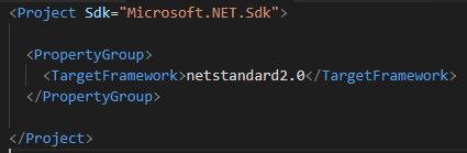
这个项目里只有一个类,也就是要被测试的类:

这个类有三个方法,分别是使用foreach,for和Linq扩展方法的Sum对集合循环并求和。
2. 使用dotnet cli建立一个console项目(如果使用VS2017的话直接建类库就可以,因为VS2017内置Test Runner),这个是测试项目,它的版本只能是2.0(可能是因为我电脑sdk的版本较老):

另外还需要引用被测试项目。
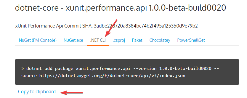
3.然后,按照官方文档安装两个库。
xUnit-Performance目前还处于Beta阶段,这两个库需要按照官网的指示进行安装:
最新版的xunit.performance.api.dll, 这里用到的是MyGet: https://dotnet.myget.org/feed/dotnet-core/package/nuget/xunit.performance.api#.
然后是最新版的 Microsoft.Diagnostics.Tracing.TraceEvent, 这个使用Nuge: https://www.nuget.org/packages/Microsoft.Diagnostics.Tracing.TraceEvent

OK,现在依赖库都装好了。
编写性能测试
性能测试和单元测试略有不同, 性能测试是跑很多次, 然后取平均值. 同时也要考虑到内存等其它因素的影响.
在性能测试里就不需要测试功能的正确性了, 但是程序在压力下可能会产生不同的结果, 尤其是多线程的情况. 这时你就需要写压力测试了.
而对于性能测试, 我们只考虑速度.
由于我是用的是dotnet cli和VSCode,所以测试项目我选用的是控制台项目,它的Main方法需要这样写:
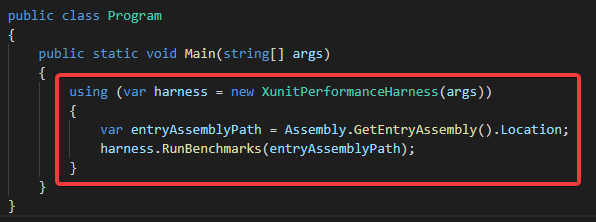
如果您能成功的使用VS2017建立测试项目,那么就不需要Main方法了,建立一个类库项目即可,直接使用VS2017的Test Runner即可。
性能测试代码
下面我们编写性能测试方法。
首先在测试项目建立一个类,然后做一些准备工作:

这里我准备了一个List<KeyValuePair<int, double>>,它有100000条数据,是随机生成的。
然后是测试方法,在这里我们使用[Benchmark]替代了xUnit单元测试中的[Fact]:

xUnit.Performance的测试会跑很多次,结果是取平均值的。
这里我们循环遍历Benchmark.Iterations,它有一个默认值,我这里默认是跑了1000次循环。
再循环里,首先您可以做一些准备工作。然后使用iteration.StartMeasurement()来开始进行测量。
只有iteration.StartMeasurement()后边的部分才会被测量,在大括号里面写被测试相关的代码就可以了。
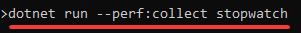
然后在命令行输入运行测试:
测试结果如下:

提供了控制台输出,xml,csv,md输出(在项目文件夹里)。
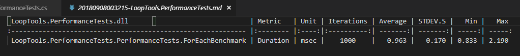
从控制台可以看到该测试的循环跑了1000次,平均结果是0.963毫秒。
下面是csv结果的截图:

下面是md结果文件的截图:
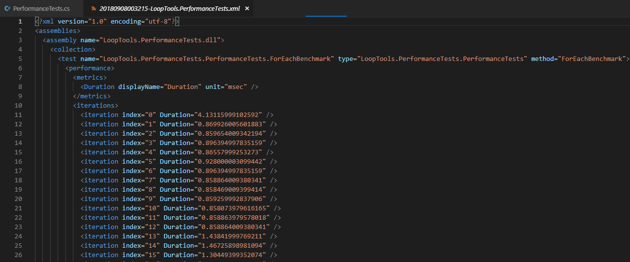
下面是xml结果文件的截图,它里面有详细数据:
内部循环
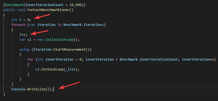
xUnit.Performance还可以添加一个内部循环属性 InnerIterationCount。先看代码,添加以下方法:

[Benchmark(InnerIterationCount = 10_000)],这里的InnerIterationCount是内部循环遍历的次数。
在StartMeasurement()之后,进行内部循环。
这样的话,外层循环的次数可能会很少,而且第一次外层循环是热身,不包括在测试结果中。
而内部循环适合于运行比较快速的代码(微秒级)。
有时确实需要这样两层循环,做一些热身工作或者需要完成不同级别的准备工作。
然后我们来跑测试
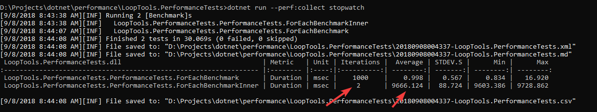
在结果里看到外层循环有2次的记录,但是它实际跑了3次,第一次算作热身,不做统计。
它的时间是内层循环的总和,除以10000之后,和第一个方法的结果差不太多。
我可以在方法中打印输出循环次数:
其结果如下:
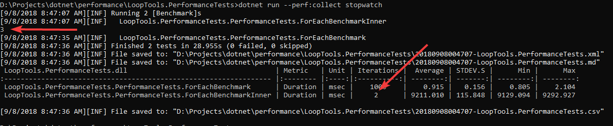
可以看到确实是跑了3次,但统计了2次。
然后我再添加另外两个测试方法,分别测试另外两个方法:

运行测试:

可以看到现在这4个测试方法的结果。
看来针对List来说foreach要比linq和for循环快。
注意foreach测试的外层循环跑了2次,而for和linq的测试循环只跑了1次,可能是因为花费时间太久了吧?这个我不太确定。
StopWatch

可以看到测试命令的参数 stopwatch,它应该是来自System.Diagnostics命名空间下的StopWatch类。
它有Start()和Stop()方法和一些其它属性用来统计逝去的时间。
StopWatch类是跨平台的,但是在其它系统上,它只能统计时间;而在Windows上,它还可以使用内核ETW events和CPU性能计数来给您更多的数据,具体请查阅相关资料。
结语
该库还有很多功能和命令的参数,具体请参考文档:https://github.com/Microsoft/xunit-performance
但是要注意,它仍然是beta状态,只能在MyGet而不是Nuget获取。

A DB2 Performance Tuning Roadmap
a db2 performance tuning roadmap
庖丁为文惠君解牛,手之所触,肩之所倚,足之所履,膝之所踦,砉然向然,奏刀騞然,莫不中音。合于《桑林》之舞,乃中《经首》之会。 文惠君曰:“嘻,善哉!技盖至此乎?
说起DB2,大家可能比较陌生,更多的是对oracle,SQLserver,MYSQL以及大行其道的NOSQL如MongoDB,REDIS等了解的比较多。笔者由于工作的原因对DB2接触的比较多,在这里谈一下自己的理解。由于笔者自身的局限性,对很多问题的描述可能准确,欢迎指正。 大家都知道MYSQL是单进程多线程,ORACLE在Window和linux上表现不同,windows下是单进程多线程,linux下是多进程方式提供服务。DB2也是以类似多地址空间(与进程相类似)的方式提供服务。
<b>Architected around the address space Conceptually, DB2 is a relational database management system. Physically, DB2 is an amalgamation of address spaces and intersystem communication links that, when adequately tied together, provide the services of a relational database management system.</b>
原文
DB2 的这种进程处理方式,OVERHEAD便是进程间通信,引入了很多的子线程的分类,如CICS THREAD,ALLIED ADDRESS SPACE,DATABASE ACCESS THREAD,这些概念可能通过进程间通信这种方式来理解就比较好接受了,这也引入了所谓的不同的CALL ATTACHEMENT FACILITY的概念,其实都是由于DB2对外开放的不同API而已。 关于DB2 cluster的工作方式更多的是DB2 DATA SHARING,可以参考
- 浅析DB2 中的DBMS CLUSTER技术
- DBMS-DSG初探之XCF
- DSG CF 之cache 漫谈
- DSG CF 之cache 漫谈1
- DSG CF 之cache 漫谈2
- DB2 Buffer 原理简介
- 数据库设计的理论依据
OUTLOOK OF PERFORMANCE
本篇内容是在写完系统调优的基本功后,在次进行的梳理,同时增加了应用调优的部分。知识的学习本身也是一个循序渐进的过程。 首先我们需要明确性能的概念,何为性能,它对应的英文单词为performance,维基百科给出的解释--- 计算机完成某项有用的工作所消耗的时间与资源WIKI。所以好的高性能,也就意味着使用更少的资源,更快的完成工作。 性能的目标是没有蛀牙,哈哈
- realistic 即性能在当前的技术下可以实现,如交易平均响应时间0.1就是可以实现的,0.000001,NOT REALISTIC
- reasonable 合理的
- quantifiable 可以量化的如RATIO,PERCENTAGES,NUMBERS,而不是good,perfect,这种空洞的描
- measurable 可以度量的
根据国情,所有这些都是要满足leader的需求为前提,指定上述目标后,就是monitor,看看当前的系统是否满足上去要求,从而进行调优。monitor根据执行的频度有三种:
- routine monitoring
- online/realtime event monitoring
- exception monitoring
其实DBA面对更多的是2,3所发现的问题,时间紧,任务重,如果可以规避还好,如果不能规避,需要实施紧急变更。但是如果monitor 1 基础打得好,可以提前发现很多问题,将问题消灭在萌芽状态。monitor 1 更多是收集性能信息,以及系统整体的运行情况。
总体指导思想
- TOP-DOWN TUNEING
- DEVIDE AND CONQUER
- 二八原则。花80%的时间解决20%的问题,带来80%的收益,即最佳性价比
- 一个前提:当系统运行或是应用出现问题的时候,我们总是假定这是一个由量变到质变的过程[变更除外,这种情况下需要紧急回退],即我们总是假设系统或是应用在以前是正常的,我们需要一个benchmark.这就给我提供了一个思路,当你没有思路时,你可以和历史数据进行比较,从而发现问题
- 关于定性和定量的问题,相对来说,定性容易,定量有时候还是比较困难的
- 从管理的角度,调优是一个持续改进的过程,应该是一个闭环,即监控发现问题,分析问题,解决问题,而后继续监控
-
一点体会: 其实调优本身也是一个资源配置的问题,在特定的场景之下,如何把有限的资源进行有效的配置,从而达到组织的目的。 整个组织目前拥有的资源,这里只对计算机系统调优而言:
- CPU
- IO
- LOCKING
- STORAGE5. human resource 当然就是你了
- NETWORKING 可忽略
- SYSTEM HARDWARE & OTHER SOFTWARE SUCH AS CICS/ZOS/CFCC
影响这些resource的方式不外乎:
1. got enough 2. not enouth 3. too much 4. inefficient 5. what are the available controls? (fixes)
两大方向
系统调优 应用调优
系统调优
关于系统调优前面已经介绍过了--系统调优的基本功,这里的任务就是如何在总结提炼.那篇文章介绍的更多内容其实对应的是routine monitor,
CICS性能数据收集交易性能数据对应的SMF 类型为110,对应的分析工具CICS PA
SMF Type 110 (subtype0) — CICS Journal Record SMF Type 110 (subtype1) — CICS Monitoring Record SMF Type 110 (subtype2) — CICS Statistics Record
DB2 SMF 对应的SMF TYPE 为100,101,102,其中
SMF TYPE=100 DB2 SUBSYSTEM STATISTICSSMF TYPE=101 DB2 ACCOUNTING SMF TYPE=102 ALL OTHERE PERFORMANCE
SMF TYPE=100 的表格如下
| CLASS | DATA COLLECTED | IFCID |
|---|---|---|
| 1 | Statistics data | 1, 2, 105,106, 202, 225 |
| 2 | Installation-defined statistics record | 152 |
| 3 | Deadlock, lock escalation, group buffer pool, data set,extension information, indications of long-running URs, and active log space shortages | 172, 196, 250, 258, 261, 262, 313, 330, 335, 337 |
| 4 | DB2 exceptional conditions | 173,191-195, 203-210, 235, 236, 238, 267, 268, 343, 402 |
| 5 | DB2 data sharing statistics record | 254 |
| 6 | Storage usage details | 225 |
| 7 | DRDA location statistics | 365 |
| 8 | Data set I/O statistics | 199 |
SMF 本身的结构也是一个树形层级结构,如果打算收取某一类型的trace,你需要关注三个方面,
- TRACE TYPE
- CLASS
- IFCID
这样对应的收取trace的命令就很好理解了
START TRACE(S) CLASS() IFCID(172) DEST(SMF) ---TNODIS TRACESTOP TRACE(S) TNO(XX) recommand defualt trace:start trace(s) c(1,3,5,6,7,8)
这里首先介绍SMF TYPE=100,由上面的表格,我们可以了解到stat报表包括的大体内容,下面我们逐一介绍,让你对报表有一个大体的了解,有时候自下而上解决不了问题的时候,stat就是一个关键的突破口。 STATISTICS 性能数据收取的时间颗粒度granularity为1分钟,相比较SMF TYPE101,102,它的量是很少。 考虑解读性能数据的重要性,后续单独写一篇来介绍,你放心,绝对值得写一章。 在结束准备工作之前,在向你介绍一个性能数据在一个颗粒度内是如何计数的,主要分为3类:
- SNOPSHOT VALUE--current value 即性能数据收取时间时对应的实时值
- HWK --HIGH WATER MARK 对应的时间颗粒度内的最高水位值
- ACCUMULATE VALUE--累加值,时间颗粒度内一个逐渐累加计数值作者注明确这一点对性能数据解读很重要。

A DB2 Performance Tuning Roadmap --DIVE INTO LOCK
a db2 performance tuning roadmap --dive into lock
在整理了db2 log相关内容的基础之上,这章整理lock的内容,相比较与log,lock的内容更多的与应用相关,涉及内容方方面面更加复杂。dbms在本质上不同于文件系统的地方在于dbms系统所支持的事务。 如果log的引入是为了保证持久化,那么lock的引入就是保证事务串行化,解决事务的并发带来了资源的race condition。不同的事务场景,定义了不同的并发需求,为此定义了4种事务的隔离级别,不同的dbms引入了不同的锁机制来实现。db2的串行化机制主要是通过lock,latch,claim/draim 来实现,具体的lock的相关属性以及lock属性对应用程序的影响比如object,size,mode,duration,participants,parameter locations都进行了介绍。当引入了dbms cluster(db2中为data sharing group,而oracle中为oracel rac) 以后,为了处理不同不同member之间数据的一致性,db2引入了physical lock以及cf lock strture 来实现全局lock 冲突检测。单个subsystem中,主要的冲突有timeout,deadlock,在datasharing group,引入了新的contention,xes contention,false contention,global lock contention。引入lock的同时不可避免的带来了新的overhead,db2主要通过irlm,xes,cf等处理锁资源的请求,除了地址空间除了锁请求之外,由于应用本身设计不合理或是某些特定的场景带来了很多问题,如temeout,deadlock,lock escalation等,如何有效的避免这些问题,需要系统运维人员以及开发人员共同努力。
本文的行文脉络基于个人对dbms lock的认知层次,行文的逻辑性,合理性,整理内容的知识面的广度和深度都有待进一步的思考。
这篇博客从落笔到完成大体的框架,持持续续时间已经接近2周,应该是自己耗时最长的一篇博客,纵使如此,每一次查看,发下仍有新的东西需要自己补充,等后续会继续补充自己的理解。
- LOCK OVERVIEW
- WHY LOCKS ? DB2 Serialization Mechanisms
- Data Consistency And Database Concurrency
- Phenomena Seen When Transactions Run Concurrently
- Lost Updates
- DIRTY READS
- Non-Repeatable Reads
- Phantoms
- Data Consistency And Database Concurrency
- LOCK PROPERTIES
- LOCK OBJECT OWNER
- LOCK PARTICIPANTS
- LOCK SIZE
- LOCK MODE
- LOCK DURATION
- LOCK REQUEST AND RELEASE
- LOCK AND TRAN ISOLATION LELVEL
- LOCKING PARAMETERS LOCATIONS
- DDL
- DML
- Precompiler Locking Parameters
- Bind Locking Parameters
- Zparm Locking Parameters
- CLAIM AND DRAIN
- LATCH
- ADVANCED TOPICS
- L-LOCK(EXPLICIT HIERARCHICAL LOCKING )EHL
- PHYSICAL LOCK
- RETAINED LOCKS(UPDATE LOCKS)
- IMPACT OF Retained LOCKS
- LOCK SCOPE:
- LOCAL LOCK
- GLOBAL LOCK
- GLOBAL LOCK COMMUNICATION
- Page Set P-Lock Negotiation
- CF LOCK STRUCTURE
- MODIFIED RESOURCE LIST(MRL)
- LOCK TABLE
- XCF
- XES
- XES CONTENTION
- FALSE CONTENTION
- GLOBAL CONTENTION
- DATA SHARING ACTIVITY REPORT
- Lock Structure Shortage Actions
- Types of locking problems
- How do I find out I have a problem
- Analyzing concurrency problems --TOOLBOXS
- DB2 commands and EXPLAIN
- DB2 TRACES
- EXAMPLE:Analysis of a simple deadlock scenario and solution
- DBD is locked
- WHY LOCKS ? DB2 Serialization Mechanisms
LOCK OVERVIEW
WHY LOCKS ?DB2 Serialization Mechanisms
Data Consistency And Database Concurrency
DBMS区别与文件系统的最本质区别:DBMS支持事务
DBMS :Allowing multiple users to access a database simultaneously without compromising data integrity.
A transaction (or unit of work)is a recoverable sequence of one or more SQL operations that are grouped together as a single unit, usually within an application process.
One of the mechanisms DB2 uses to keep data consistent is the transaction. A transaction or(otherwise known as a unit of work) is a recoverable sequence of one or more SQL operations that are grouped together as a single unit, usually within an application process. The initiation and termination of a single transaction defines points of data consistency within a database; either the effects of all SQL operations performed within a transaction are applied to the database and made permanent (committed), or the effects of all SQL operations performed are completely "undone" and thrown away (rolled back).
Phenomena Seen When Transactions Run Concurrently
事务并发带来的问题,为了解决这些问题,DB2定义了4种事务隔离级别。
- LOST UPDATE
- DIRTY READS
- NON-REPEATABLE READS
- PHANTOMS
Lost Updates
Occurs when two transactions read the same data, both attempt to update the data read, and one of the updates is lost
Transaction 1 and Transaction 2 read the same row of data and both calculate new values for that row based upon the original values read. If Transaction 1 updates the row with its new value and Transaction 2 then updates the same row, the update operation performed by Transaction 1 is lost
DIRTY READS
Occurs when a transaction reads data that has not yet been committed
Transaction 1 changes a row of data and Transaction 2 reads the changed row before Transaction 1 commits the change. If Transaction 1 rolls back the change, Transaction 2 will have read data that theoretically, never existed.
Non-Repeatable Reads
Occurs when a transaction executes the same query multiple times and gets different results with each execution
Transaction 1 reads a row of data, then Transaction 2 modifies or deletes that row and commits the change. When Transaction 1 attempts to reread the row, it will retrieve different data values
Phantoms
Occurs when a row of data that matches some search criteria is not seen initially
Transaction 1 retrieves a set of rows that satisfy some search criteria, then Transaction 2 inserts a new row that contains matching search criteria for Transaction 1’s query. If Transaction 1 re-executes the query that produced the original set of rows, a different set of rows will be retrieved – the new row added by Transaction 2 will now be included in the set of rows returned
LOCK PROPERTIES
LOCK OBJECT OWNER
这里的object是指锁所施加的对象,不同的锁所能适用的对象是不同的。如PAGE LOCK的对象肯定是PAGE.
OWNER 表示谁持有锁,有的是TRAN,有的是DB2 MEMBER
LOCK PARTICIPANTS
Locking is a complex interaction of many parts.
- DBM1, where SQL executes, is the beginning of locking.
- The IRLM, a separate address space, is where locks are held and managed. The DBM1 AS requests locks from the IRLM. In addition to its functionality of granting and releasing locks, the IRLM is also in charge of detecting deadlock and timeout situations.
- In a data sharing environment, there are two other ingredients in the soup. The XCF address space is where its XCF component resides. The XES does some lock management and communicates directly with the lock structure in the coupling facility
LOCK SIZE
访问数据的范围
设计锁的颗粒度对系统和应用均有影响:设计时要综合考虑- 锁本身也是一种资源,持有的lock size越大,锁资源消耗越小
- lock size的大小与对应用访问的并发(concurrent)成反比关系
- LOCK SIZE 带来的另外一个副作用就是当你申请的锁资源足够多,以至于超过系统设定的阀值时(NUMLKUS/NUMLKTS/LOCK MAX =0,SYSTEM,N),
lock size: PAGE/ROW /TABLE /PARENT LOCKS:TABLESPACE /PARTITIONINTENT LOCKS:IS/IX USED whenever page or row locks are being usedPage/Row locks are not compatible with tablespace locks The solution is "Intent Locking" Regardless of the locksize, DB2 will always start with a tablespace lock
登录后复制
GROSS LOCKS:The gross locks (S, U, SIX and X) are tablespace locks which are used in three
situations - lock size tablespace
- lock table for a non-segmented tablespace
- lock escalation for a non-partitioned tablespace
LOCK MODE
数据的访问方式:独占还是共享 S/U/X
X:exclusive, not sharable with other
S:shared, sharable with other S-locks
LOCK MODE之间的兼容性如下:S U X S Y Y N U Y N N X N N N LOCK DURATION
持有数据的时间:commit,across commit(with hold)
FROM:START OF FIRST USE
TO :COMMIT OR MOMENTIALIY
LOCK REQUEST AND RELEASE
When modifying data (Insert, Update and Delete),DB2 determines all locking actions
- Lock size Tablespace
=> lock is taken at first use
=> lock is released at commit or deallocate - SQL- Statement “Lock Table … in Exclusive Mode”
=> initially an IX-lock (on the tablespace)
=> lock is taken at first use
=> lock is released at commit or deallocate - Page lock and row lock
=> initially an IX-lock (on the tablespace)
=> then X-locks are taken on each page/row as needed
=> these X-locks are released at commit
LOCK AND TRAN ISOLATION LELVEL
每一种事务隔离级别锁所能解决的问题
- Repeatable Read
=> locks all data read by DB2
=> guarantees that exact the same result set will be returned when reusing the cursor - Read Stability
=> locks all data “seen” by the application
=> guarantees that at least the same result set will be returned when reusing the cursor - Uncommitted Read (UR)
Pro:
Our read will be “cheaper”
We are not disturbing others
Con:
We may read data
which may be “un-inserted”
which may be “un-updated”
When you are reading live (operational) data,you can never guarantee exact results - Cursor Stability (CS)
=> a lock is taken when the row is fetched
=> the lock is released when next row is fetched,
or at end of data or at Close Cursor
For page locks:
=> a lock is taken when the first row on the page is fetched
=> the lock is released when next page is fetched,
or at end of data or at Close Cursor
This means:When you have fetched a row and have not reached end of data or closed the cursor,
you are holding an S-lock on the row or page - LOCK AVOIDANCE
UpdateableRead-OnlyDECLARE upd_cur CURSOR FOR SELECT data1, data2 FROM table FOR UPDATE OF colx
登录后复制AmbiguousDECLARE ro_cur CURSOR FOR SELECT DEPTNO, AVG(SALARY) FROM EMP GROUP BY DEPTNO
登录后复制=> Use FOR READ ONLY or FOR FETCH ONLYDECLARE amb_cur CURSOR FOR SELECT data1, data2 FROM table
登录后复制
If we have the following:
Read-Only (or Ambiguous) Cursor
Cursor Stability
Currentdata No
it is possible that we can get "Lock Avoidance“
Lock avoidance is advantageous!
A possible problem with Currentdata No:
Fetch a row
...
Update (or Delete) Where Key = :hostkey
can give SQLSTATE="02000" (Not Found)
LOCKING PARAMETERS LOCATIONS
下面分别介绍了系统参数,应用参数如何影响LOCK行为
DDL
OBJECT DEFINITION,CREATE TABLESPACE:
- LOCKMAX (INTEGER,SYSTEM)
- LOCKSIZE
DEFAULT:ANY
OPTION:ANY,TABLESPACE,TABLE,PAGE,ROW,LOB - MAXROW: INTEGER
DEFAULT:255
USED TO increase concurrency
MAXROWS 1Used to emulate row-level locking
locking without the costs of page p-lock processing - MEMBERCLUSTER:(P-LOCK)
Clustering per member
Reduce p-lock contentions forspace mappages
Destroys clustering according to clustering index - TRACKMOD (P-LOCK)
DEFAUTL:NO
OPTION:YES/NO
DML
- LOCK TABLE
SYNTAX:LOCK {TABLE, TABLESPACE [partno]} IN
{EXCLUSIVE, SHARE} MODE - Cursor Definitions
FOR UPDATE OF
FOR READ ONLY- Tells DB2 the result set is read-only
- Positioned UPDATEs and DELETEs are not allowed
- No U or X locks will be obtained for the cursor
- Isolation Clause
WITH [UR, CS, RS, RR]- USE AND KEEP EXCLUSIVE LOCKS
- USE AND KEEP UPDATE LOCKS
- USE AND KEEP SHARE LOCKS
Precompiler Locking Parameters
NOFOR Option:NO FOR update clause mandatory for positioned updates
STDSQL(YES): Implies NOFOR
Bind Locking Parameters
- CURRENTDATA
FUNCTION:CURRENTDATA helps to determine if DB2 will attempt to avoid locks
mean:Must the data in program be equal to the data at the current cursor position
lock aovidance
demo:
CURRENTDATA(NO)
note - ISOLATION
- RELEASE
Zparm Locking Parameters
| ZPARM | MEANING |
|---|---|
| URCHKTH | UR Checkpoint Frequency Threshold |
| URLGWTH | UR Log Write Threshold |
| LRDRTHLD | Long-Running Reader |
| RELCURHL | Release Held Lock |
| EVALUNC | Evaluate Uncommitted |
| SKIPUNCI | Skip Uncommitted Inserts |
| RRULOCK | U lock for RR/RS |
| XLKUPDLT | X lock for searched U/D |
| NUMLKTS | Locks per Table(space) |
| NUMLKUS | Locks per User |
CLAIM AND DRAIN
BETWEEN SQL AND SQL:DB2 USE LOCKS
BETWEEN UTILITY AND SQL:DB2 USE CLAIM AND DRAIN
BASE:
FOR EACH OBJECT(TABLESPACE,PARTITION,TABLE,IDNEXSPACE),THERE IS A CLAIM-COUNT
WHICH IS INCREASED 1 AT START AND DECREASE BY 1 AT COMMIT
A utility starts with a Drain
No new Claims are allowed (wait, maybe timeout)
If the Claim-count >0 the utility waits (maybe timeout)
When the Claim-count reaches zero, the utility can continue
Two important situations:
- UR (Uncommitted Read) takes no locks – but increases Claim-count (UR REQUEST MASS-DELETE LOCKS)
- For Cursor With Hold the Claim-count is not reduced at Commit
A claim is a notification to DB2 that a particular object is currently being accessed. Claims usually do not continue to exist beyond the commit point one exception being a Cursor with Hold. In order to access the DB2 object within the next unit of work, an application needs to make a new claim.Claims notify DB2 that there is current interest in or activity on a DB2 object.Even if Uncommitted Read doesn’t take any locks, a claim is taken. As long as there are any claims on a DB2 object, no drains may be taken on the object until those claims are released.
登录后复制
A drain is the action of obtaining access to a DB2 object, by:Preventing any new claims against the object.Waiting for all existing claims on the object to be released.
A drain on a DB2 object causes DB2 to quiesce all applications currently claiming that resource, by allowing them to reach a commit point but preventing them (or any other application process) from making a new claim.A drain lock also prevents conflicting processes from trying to drain the same object at the same time.
Utilities detect claimers are present and wait
Drain Write waits for all write claims to be released
Drain All waits for claims on all classes to be released
SHRLEVEL(CHANGE) Utilities are CLAIMers
LATCH
Latches – managed by DB2
? BM page latching for index and data pages
? DB2 internal latching (many latches grouped into 32 latch classes)
? Latches – managed by IRLM
? Internal IRLM serialization
ADVANCED TOPICS
虽然标题是advanced topics,其实涉及的内容并没有本质的区别,只不过我们在看待问题,分析问题时需要从单个DB2 SUBSYSTEM的视角上升到DBMS CLUSTER的高度,即DATA SHARING GROUP的高度。为了处理不同的member之间共享数据的COHERENCY问题,DB2引入P-LOCK,区别主要在于单个DB2 SUBSYSTEM中的LOCK owner均为tran,而P-LOCK的owner为DB2 SUBSYSTEM.因此这里的内容按照这种分类进行介绍L-LOCK,P-LOCK,RETAINED LOCK,这几种锁之间的区别需要了解。
L-LOCK(EXPLICIT HIERARCHICAL LOCKING )EHL
特点:
THE KIND YOU HAVE IN BOTH DATA SHARING AND NON DATA SHARING SUBSYTEM THEN CONTROL DATA CONCRRRENCY OF ACCESS TO OBJECTS THEN CAN BE LOCAL OR GLOBAL THEY ASSOTIATED WITH PROGRAMS
WHY IS HIERACHICAL
SO THE MEMBER DB2 SUBSYSTEM WILL NOT PROPAGATE L-LOCKS TO THE CF UNNECESSARILY
- PARENT LOCK
PARENT LOCK ARE TABLE SPACE LOCKS OR DATA PARTITION LOCK
GROSS LOCKS ARE ALWAYS GLOBAL LOCKS - CHILD LOCK
PAGE /ROW LOCK
EXCEPTION: MAYBE TABLES LOCKS IF SEGMENT TABLESPACE
PAGE/ROW LOCK CAN BE GRANTED LOCALLY IF NOT IN INTER-DB2 R/W SHARING STATE
ASYNCHRONOUS CHILD PROPAGATION WHEN INTER-SYTEM INTEREST FIST OCCUR - L-LOCK PROPAGATION
NOT ALL L-LOCKS ARE PROPAGATED TO THE DB2 LOCK STRUCTURE
PARENT L-LOCKS ARE ALMOST ALWAYS PROPAGATE TO THE DB2 LOCK STRUCTURE - Child Locks Propagation based on Pageset P-lock
Now based on cached(held) state of the pageset P-lock
If pageset P-lock negotiated from X to SIX or IX, then child L-locks propagated
Reduced volatility
If P-lock not held at time of child L-lock request, child lock will be propagated
"Index-only" scan (if any locks taken) must open table space
Parent L-lock no longer need to be held in cached state after DB2 failure
A pageset IX L-lock no longer held as a retained X lock
Important availability benefit in data sharing
CHILD L-LOCKS ARE PROPAGATED TO THE DB2 LOCK STRUCTURE ONLY IF THERE IS INTER DB2 PARENT L-LOCKS CONFICT ON A DATABASES OBJECT
PHYSICAL LOCK
特点:
EXCLUSIVE TO DATA SHARING
ARE ONLY GLOBAL
USED TO MAINTAIN DATA COHERENCY IN DATA SHARING
ALSO USED TO MAINTAIN EDMPOOL CONSISTENCY AMONG MEMBERS
ASSOTIATED BY(OWNED BY) DB2 MEMBERS
P-LOCK CAN BE NEGOTIATTED BETWEEN DB2 MEMBERS
NO TIMEOUT OR DEADLOCK DETECTION
分类
- PAGE SET P-LOCK
- PAGE P-LOCK
- PAGE SET/PARTITION CASTOUT P-LOCK
- GBP STRUCTURE P-LOCK
RETAINED LOCKS(UPDATE LOCKS)
AIM:PROTECT UNCOMMITED DATA FROM ACCESS BY THER LOCK STRUCTURE
UPDATE(IX,SIX,X)
GLOBAL LOCKS ARE RETAINED AFTER FAILTUREIMPACT OF Retained LOCKS
The ONLY way to clear retained locks is by estarting the failed DB2 subsystem.
登录后复制LOCK SCOPE:
LOCAL LOCK
GLOBAL LOCK
A LOCK THAT A DB2 SHARING DB2 MEMBERHAS TOMAKE KNOWN TO OTHERS MEMBERS OF THIS DATA SHARING GROUP
THE IRLM VIA XES,PROPAGATE TO THES LOCKS TO THE STRUCTURE IN THE CF
XCF,XES的内容在XES contention部分介绍。
GLOBAL LOCK COMMUNICATION
HOW ARE GLOBAL LOCK REQUESTS MADE KNOWN TO OTHER DB2 MEMBERS?
THEY ARE PROPAGATED TO DB2 LOCK STRUCTURE
与APPLICATION LOCK不同的是,PHYSCIAL LOCK 可以做Page Set P-Lock Negotiation。
上图展示了INERDB2 READ/WRITE INTEREST场景下的PAGE SET P-LOCK NEGOTIATION。所谓的negotiation就是锁请求方以及锁申请方将锁请求均DOWNGRADE,从而达到compatible的目的。需要注意的是,PAGE SET P-LOCK STATE状态的变化需要涉及IRLM以及XCF通讯机制。PAGE SET P-LOCK对GLOBAL BUFFER POOL起一种标志作用,
对于READ的DB2 SUBSYSTEM, must register its
interest in read pages in the GBP directory
对于UPDATER的DB2 SUBSYSTEM,must write updated pages to the group buffer pool and register those updated pages in the GBP directory
CF LOCK STRUCTURE
DEVIDE INTO TWO PARTS OF CF LOCK STRUCTURE RATIO OF LAST TWO COMPONETS DEFAULT ROUGHLY 50%CAN BE ALTERED BY IRLM PARAMETER
MODIFIED RESOURCE LIST(MRL)
OVERVIEW OF MRL STRUCTURE
ACTIVEstatus of active means that the DB2 system is running.
Retained, on the other hand, means that a DB2 and/or its associated IRLM has failed
CONTAINS ENTRIES FOR ALL CRURENTLY HELD MODIFY LOCKS
IN THE EVENT OF DB2 FAILTURE ENSURE THAT OTHER MEMBER OF DB2 KNOW WHICH LOCKS MUST BERETIANED
It is essentially a list structure that lists all the update or modify locks in the data sharing group
DISPLAY GROUP ; Display “LIST ENTRIES IN USE”
NUMBER LIST ENTRIES : 7353, LIST ENTRIES IN USE: 1834
WARNING: When the LIST ENTRIES IN USE catches up to the NUMBER LIST ENTRIES, new modify lock requests will not be granted, and transactions will begin to fail with -904s.
LOCK TABLE
A ''POOL'' OF HASH POINTERS
CONTAINS ENTRIES FOR ALL READ AND MODIFY LOCKS
USED FOR GLOBAL LOCK CONTENTION
It is very difficult to keep track of how full a randomly populated table is, so the only way to track its utilization is indirectly. In DB2 data sharing, that tracking mechanism is false contention
SIZE OF EACH INDIVIDUAL ENTRY SET BY MAXUSRS PARAMETER IN IRLMPROC OF FIRST IRLM JOIN THE GROUP
NUMBER OF MEMBER IN THE GROUP
XCF
其实主要的目的就是提供INTER-SUBSYTEM之间通讯的API,主要的功能有三个:
- Signaling Services provide a method for communicating between members of the same XCF roup, which is a set of related members defined to XCF by a multisystem application. This function supports the single system image concept of a parallel sysplex, both by providing communication etween subsystems, such as DB2 members, as well as z/OS components in each image.
- Group Services allow multisystem applications to define groups and their members to XCF. Group services also provide the means for requesting information about the other members in the same XCF group, using SETXCF commands.
- Status Monitoring Services of XCF provide the means for monitoring the status of other z/OS systems in the same sysplex.
XES
提供了不同的SUBSYSTEM访问CF的API。XES本身仅支持两种锁类型,即S|X类型。但是DB2 SUBSYTEMB本身支持多种不同类型的锁,这就带来一个问题,这些锁类型在上送到CF时,应该如何映射,DB2 V7 Protocol Level 1和V8 Protocol Level 2的处理差别比较大,当然这种变化的目的还是在保证能完全检测到锁冲突的前提下,减少上送到CF锁的请求次数,优化全局锁检测机制。V7到V8优化的出发点还是进一步的解决XES锁映射问题,V8到V10甚至V11基本上无变化,可见V8优化的意义之重大。
DB2在DATA SHARING 下是显式的三级锁结构,TWO LEVELS OF APPLICATION LOCKS外加DB2 member级别的PAGE SET P LOCK.
DB2 PAGE SET P-LOCK的状态变化如下图:action DB2 member interest page set p lock STAE CHANGE open PP-LOCK S/IS NONE->R/O PSEUDO OPEN PP-LOCK IX/SIX/X/U R/O->R/W PSEDUO CLOSE PP-LOCK S/IS R/W->R/O Physical CLOSE NONE R/O->NONE
产生的根源为XES本身设计时仅支持两种锁类型,
?XES Contention = XES-level resource contention as XES
only understands S or X
eg member 1 asking for IX and member 2 for IS
Big relief in V8
产生的根源主要是由于DB2 lock table定义的太小或是hash算法离散型不够好,导致不同的DB2资源hash到同一lock table hash class上而产生的冲突,可以通过放大CF lock table来解决,因此FALSE CONTENTION标志着 CF LOCK STRUCTURE的大小是否合适。
GLOBAL CONTENTIONGLOBAL CONTENTION 本身包含XES CONTENTION,FALSE CONTENTION,REAL CONTENTION,其中REAL CONTENTION 确实为资源冲突,如资源热点,其它的两种冲突是由于引入DATA SHARING 的OVERHEAD
根据上面的介绍,下面给出A DB2 Performance Tuning Roadmap-2data sharing BLOCK的一个展示
L-LOCK(SHARING)部分表明了数据共享的程度
P/L XES CONTENTION表明P-LOCK,L-LOCK中需要上送CF的比例。其中P-LOCK需要上送的大部分为PAGE P-LOCK.
Lock Structure Shortage Actions
WHEN YOU Running Out of Space in the Lock Structure:
DXR170IDJP5005 THE LOCK STRUCTURE DSNDB0G_LOCK1 IS 50%(60%,70%) IN USE
DXR142IDJP5005 THE LOCK STRUCTURE DSNDB0G_LOCK1 IS zz% IN USE
ACTION:
- Check for ‘DOWN’ DB2s holding Retained Locks
- RESTART DB2s to Reclaim Lock List Space
- Lower the Lock Escalation Values to Lower Number of Locks
- Increase Size of Lock Structure
DYNAMICALLY:SETXCF START,ALTER,STRNAME=DSNDB0G_LOCK1,SIZE=newsize Only Increases Lock List Table (MRL)REBUILDING – Two Methods:Letting IRLM
登录后复制
今天的关于hashCode method performance tuning的分享已经结束,谢谢您的关注,如果想了解更多关于(转) Ensemble Methods for Deep Learning Neural Networks to Reduce Variance and Improve Performance、.NET Core 性能分析: xUnit.Performance 简介、A DB2 Performance Tuning Roadmap、A DB2 Performance Tuning Roadmap --DIVE INTO LOCK的相关知识,请在本站进行查询。
本文标签: