本篇文章给大家谈谈用于LogisticRegression的SparkMLLibTFIDF实现,以及logisticregressionpython的知识点,同时本文还将给你拓展2017年2月14日L
本篇文章给大家谈谈用于LogisticRegression的Spark MLLib TFIDF实现,以及logisticregression python的知识点,同时本文还将给你拓展2017年2月14日 Logistic Regression、GridSearchCV的LogisticRegression无法收敛、Linear and Logistic Regression in TensorFlow、linear regression and logistic regression with pytorch等相关知识,希望对各位有所帮助,不要忘了收藏本站喔。
本文目录一览:- 用于LogisticRegression的Spark MLLib TFIDF实现(logisticregression python)
- 2017年2月14日 Logistic Regression
- GridSearchCV的LogisticRegression无法收敛
- Linear and Logistic Regression in TensorFlow
- linear regression and logistic regression with pytorch
")
用于LogisticRegression的Spark MLLib TFIDF实现(logisticregression python)
我尝试使用Spark
1.1.0提供的新的TFIDF算法。我正在用Java写MLLib的工作,但我不知道如何使TFIDF实现有效。由于某种原因,IDFModel仅接受JavaRDD作为方法转换的输入,而不接受简单的Vector。
如何使用给定的类为我的LabledPoints建模TFIDF向量?
注意:文档行的格式为[标签; 文本]
到目前为止,这里是我的代码:
// 1.) Load the documents JavaRDD<String> data = sc.textFile("/home/johnny/data.data.new"); // 2.) Hash all documents HashingTF tf = new HashingTF(); JavaRDD<Tuple2<Double, Vector>> tupleData = data.map(new Function<String, Tuple2<Double, Vector>>() { @Override public Tuple2<Double, Vector> call(String v1) throws Exception { String[] data = v1.split(";"); List<String> myList = Arrays.asList(data[1].split(" ")); return new Tuple2<Double, Vector>(Double.parseDouble(data[0]), tf.transform(myList)); } }); tupleData.cache(); // 3.) Create a flat RDD with all vectors JavaRDD<Vector> hashedData = tupleData.map(new Function<Tuple2<Double,Vector>, Vector>() { @Override public Vector call(Tuple2<Double, Vector> v1) throws Exception { return v1._2; } }); // 4.) Create a IDFModel out of our flat vector RDD IDFModel idfModel = new IDF().fit(hashedData); // 5.) Create Labledpoint RDD with TFIDF ???*肖恩·欧文(Sean Owen)的 *解决方案 :
// 1.) Load the documents JavaRDD<String> data = sc.textFile("/home/johnny/data.data.new"); // 2.) Hash all documents HashingTF tf = new HashingTF(); JavaRDD<LabeledPoint> tupleData = data.map(v1 -> { String[] datas = v1.split(";"); List<String> myList = Arrays.asList(datas[1].split(" ")); return new LabeledPoint(Double.parseDouble(datas[0]), tf.transform(myList)); }); // 3.) Create a flat RDD with all vectors JavaRDD<Vector> hashedData = tupleData.map(label -> label.features()); // 4.) Create a IDFModel out of our flat vector RDD IDFModel idfModel = new IDF().fit(hashedData); // 5.) Create tfidf RDD JavaRDD<Vector> idf = idfModel.transform(hashedData); // 6.) Create Labledpoint RDD JavaRDD<LabeledPoint> idfTransformed = idf.zip(tupleData).map(t -> { return new LabeledPoint(t._2.label(), t._1); });答案1
小编典典IDFModel.transform()如您所见,接受JavaRDD或RDD的Vector。在单个上计算模型没有任何意义Vector,所以这不是您想要的吗?
我假设您正在使用Java,因此您想将此应用到JavaRDD<LabeledPoint>。LabeledPoint包含Vector和标签。IDF不是分类器或回归器,因此不需要标签。您可以map一堆LabeledPoint来提取它们Vector。
但是你已经有了一个JavaRDD<Vector>以上。TF-
IDF仅仅是一种基于语料库中的词频将词映射到实值特征的方法。它还不输出标签。也许您的意思是想从TF-IDF衍生的特征向量以及其他一些已有的标签中开发分类器?
也许这可以解决问题,但否则,您必须极大地阐明您正在尝试使用TF-IDF实现的目标。

2017年2月14日 Logistic Regression
Logistic Regression assumes that the probability of the dependent varaiable y equaling a positive case can be interpreted as logistic function

We can now defind the cost function as
![]()
To minimize cost function, gradient descent method can be used
The process begins with computing the derivative of cost function
![]()
Then improved by repeating
![]()
import numpy as np
import pandas as pd
from sklearn.linear_model import LogisticRegression
from sklearn.model_selection import train_test_split
from pylab import scatter, show, legend, xlabel, ylabel

df = pd.read_csv("data/data.csv", header=0)
X = df[["grade1","grade2"]].as_matrix()
y = df["label"].as_matrix()
X_train, X_test, y_train, y_test = train_test_split(X, y, test_size=0.5)

# train scikit learn model
clf = LogisticRegression()
clf.fit(X_train,y_train)
print ''scikit score:'', clf.score(X_test, y_test)
#scikit score: 0.9

# visualize data
def visualize(X, y):
    pos = np.where(y == 1)
    neg = np.where(y == 0)
    scatter(X[pos, 0], X[pos, 1], marker=''o'', c=''b'')
    scatter(X[neg, 0], X[neg, 1], marker=''x'', c=''r'')
    xlabel(''Exam 1 score'')
    ylabel(''Exam 2 score'')
    legend([''Not Admitted'', ''Admitted''])
    show()

visualize(X, y)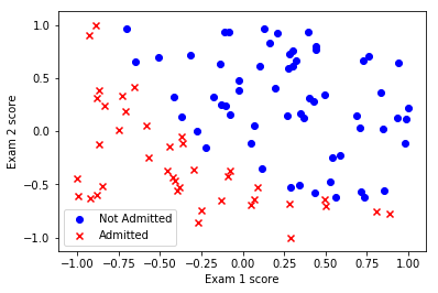
class myLogisticRegression:

    def sigmoid(self, x):
        return 1.0/(1.0+np.exp(-x))

    def logistic(self, X, theta):
        return self.sigmoid(np.dot(X, theta))

    def cost(self, X, y, theta):
        m = X.shape[0]
        return -1.0 / m * (np.dot(y, np.log(self.logistic(X, theta))) + np.dot((1-y), (1-self.logistic(X, theta))))

    def derivative_of_cost(self, X, y, theta):
        m = X.shape[0]
        return 1.0 / m * np.dot(self.logistic(X, theta)-y, X)

    def gradient_descent(self, X, y, theta, alpha):
        return theta - alpha * self.derivative_of_cost(X, y, theta)

    def fit(self, X, y, alpha, num_iter):
        self.theta = np.zeros(X.shape[1])
        for i in range(num_iter):
            self.theta = self.gradient_descent(X, y, self.theta, alpha)

    def predict(self, X):
        return self.logistic(X, self.theta)

    def score(self, X, y):
        return 1.0 - 1.0 * np.count_nonzero(np.round(self.predict(X)) - y) / len(y)


lr = myLogisticRegression()
lr.fit(X_train, y_train, .1, 1000)
print ''score:'', lr.score(X_test, y_test)
#score: 0.86

GridSearchCV的LogisticRegression无法收敛
如何解决GridSearchCV的LogisticRegression无法收敛?
我正在寻找逻辑回归的最佳参数,但是我发现“最佳估计量”并没有收敛。
是否有一种方法可以指定估算器需要收敛才能考虑在内?
这是我的代码。
# NO PCA
cv = GroupKFold(n_splits=10)
pipe = Pipeline([(''scale'',StandardScaler()),(''mnl'',LogisticRegression(fit_intercept=True,multi_))])

param_grid = [{''mnl__solver'': [''newton-cg'',''lbfgs'',''sag'',''saga''],''mnl__C'':[0.5,1,1.5,2,2.5],''mnl__class_weight'':[None,''balanced''],''mnl__max_iter'':[1000,2000,3000],''mnl__penalty'':[''l1'',''l2'']}]

grid = gridsearchcv(estimator = pipe,param_grid=param_grid,scoring=scoring,n_jobs=-1,refit=''neg_log_loss'',cv=cv,verbose=2,return_train_score=True)

grid.fit(X,y,groups=data.groups)


# WITH PCA
pipe = Pipeline([(
    (''scale'',(''pca'',PCA())
    (''mnl'',mnl)])

param_grid = [{''pca__n_components'':[None,15,30,45,65]
            ''mnl__solver'': [''newton-cg'',scoring=''neg_log_loss'',refit=True,verbose=2)

grid.fit(X,groups=data.groups)
在第一种情况下,发现的最佳估计量是使用l2-lbfgs求解器,经过1000次迭代,并且收敛。第二个方法是找到的最佳估计器,它是使用saga求解器和l1罚函数进行的3000次迭代。我觉得这与求解器有关...但是无论如何,是否有一种简单的方法可以说明它必须收敛才能接受为最佳算法?
解决方法
暂无找到可以解决该程序问题的有效方法,小编努力寻找整理中!
如果你已经找到好的解决方法,欢迎将解决方案带上本链接一起发送给小编。
小编邮箱:dio#foxmail.com (将#修改为@)

Linear and Logistic Regression in TensorFlow
Linear and Logistic Regression in TensorFlow
Graphs and sessions
TF Ops: constants, variables, functions
TensorBoard
Lazy loading
Linear Regression: Predict life expectancy from birth rate
Let''s start with a simple linear regression example. I hope you all are already familiar with linear regression. If not, you can read about it on Wikipedia. Basically, we''ll be building a very simple neural network consisting of one layer to infer the linear relationship between one explanatory variable X and one dependent variable Y.
Problem
I recently came across the visualization of the relationship between birth rates and life expectancies of different countries around the world and found that fascinating. Basically, it looks like the more children you have, the younger you are going to die! You can play the visualization created by Google based on the data collected by the World Bank here.
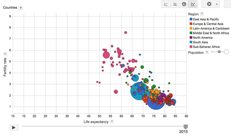
My question is, can we quantify that relationship? In other words, if the birth rate of a country is and its life expectancy is , can we find a linear function f such that ? If we know that relationship, given the birth rate of a country, we can predict the life expectancy of that country.
For this problem, we will be using a subset of the World Development Indicators dataset collected by the World Bank. For simplicity, we will be using data from the year 2010 only. You can download the data from class''s GitHub folder here.
Dataset Description
Name: Birth rate - life expectancy in 2010
X = birth rate. Type: float.
Y = life expectancy. Type: foat.
Number of datapoints: 190
Approach
First, assume that the relationship between the birth rate and the life expectancy is linear, which means that we can find w and b such that .
To find w and b (in this case, they are both scalars), we will use backpropagation through a one layer neural network. For the loss function, we will be using mean squared error. After each epoch, we measure the mean squared difference between the actual value Ys and the predicted values of Ys.
You can download the file examples/03_linreg_starter.py from the class''s GitHub repo to give it a shot yourself. After you''re done, you can compare with the solution below. You can also visit examples/03_linreg_placeholder.py on GitHub for the executable script.
import tensorflow as tf
import utils
DATA_FILE = "data/birth_life_2010.txt"
# Step 1: read in data from the .txt file
# data is a numpy array of shape (190, 2), each row is a datapoint
data, n_samples = utils.read_birth_life_data(DATA_FILE)
# Step 2: create placeholders for X (birth rate) and Y (life expectancy)
X = tf.placeholder(tf.float32, name=''X'')
Y = tf.placeholder(tf.float32, name=''Y'')
# Step 3: create weight and bias, initialized to 0
w = tf.get_variable(''weights'', initializer=tf.constant(0.0))
b = tf.get_variable(''bias'', initializer=tf.constant(0.0))
# Step 4: construct model to predict Y (life expectancy from birth rate)
Y_predicted = w * X + b
# Step 5: use the square error as the loss function
loss = tf.square(Y - Y_predicted, name=''loss'')
# Step 6: using gradient descent with learning rate of 0.01 to minimize loss
optimizer = tf.train.GradientDescentOptimizer(learning_rate=0.001).minimize(loss)
with tf.Session() as sess:
# Step 7: initialize the necessary variables, in this case, w and b
sess.run(tf.global_variables_initializer())
# Step 8: train the model
for i in range(100): # run 100 epochs
for x, y in data:
# Session runs train_op to minimize loss
sess.run(optimizer, feed_dict={X: x, Y:y})
# Step 9: output the values of w and b
w_out, b_out = sess.run([w, b])
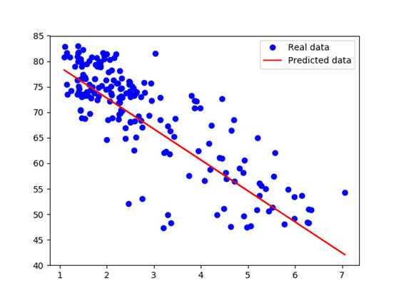
After training for 100 epochs, we got the average square loss to be 30.04 with w = -6.07, b = 84.93. It confirms our belief that there''s a negative correlation between the birth rate and the life expectancy of a country. And no, it doesn''t mean that having a child takes off 6 years of your life.
You can make other assumptions about the relationship between X and Y. For example, if we have a quadratic function:
To find w, u, and b for this model, we only have to add another variable u and change the formula for Y_predicted.
# Step 3: create variables: weights_1, weights_2, bias. All are initialized to 0
w = tf.get_variable(''weights_1'', initializer=tf.constant(0.0))
u = tf.get_variable(''weights_2'', initializer=tf.constant(0.0))
b = tf.get_variable(''bias'', initializer=tf.constant(0.0))
# Step 4: predict Y (number of theft) from the number of fire
Y_predicted = w * X * X + X * u + b
# Step 5: Profit!
Control flow: Huber loss
Looking at the graph, we see that several outliers on the central bottom are outliers: they have low birth rate but also low life expectancy. Those outliers pull the fitted line towards them, making the model perform worse. One way to deal with outliers is to use Huber loss. Intuitively, squared loss has the disadvantage of giving too much weights to outliers (you square the difference - the larger the difference, the larger its square). Huber loss was designed to give less weight to outliers. Wikipedia has a pretty good article on it. Below is the Huber loss function:

To implement this in TensorFlow, we might be tempted to use something Pythonic such as:
if tf.abs(Y_predicted - Y) <= delta:
# do something
However, this approach would only work if TensorFlow''s eager execution were enabled, which we will learn about in the next lecture. If we use the current version, TensorFlow would soon notify us that "TypeError: Using a `tf.Tensor` as a Python `bool` is not allowed." We will need to use control flow ops defined by TensorFlow. For the full list of those ops, please visit the official documentation.
Control Flow Ops
tf.count_up_to, tf.cond, tf.case, tf.while_loop, tf.group ...
Comparison Ops
tf.equal, tf.not_equal, tf.less, tf.greater, tf.where, ...
Logical Ops
tf.logical_and, tf.logical_not, tf.logical_or, tf.logical_xor
Debugging Ops
tf.is_finite, tf.is_inf, tf.is_nan, tf.Assert, tf.Print, ...
To implement Huber loss, we can use either tf.greater, tf.less, or tf.cond. We will be using tf.cond since it''s the most general. Other ops'' usage is pretty similar.
tf.cond(
pred,
true_fn=None,
false_fn=None,
...)
This basically means that if the condition is true, use the true function. Else, use the false function.
def huber_loss(labels, predictions, delta=14.0):
residual = tf.abs(labels - predictions)
def f1(): return 0.5 * tf.square(residual)
def f2(): return delta * residual - 0.5 * tf.square(delta)
return tf.cond(residual < delta, f1, f2)
With Huber loss, we found w: -5.883589, b: 85.124306. The graph compares the fitted line obtained by squared loss and Huber loss.

Which model performs better? Ah, we should have had a test set.
tf.data
You can visit examples/03_linreg_dataset.py on GitHub for the executable script.
According to Derek Murray in his introduction to tf.data, a nice thing about placeholder and feed_dicts is that they put the data processing outside TensorFlow, making it easy to shuffle, batch, and generate arbitrary data in Python. The drawback is that this mechanism can potentially slow down your program. Users often end up processing their data in a single thread and creating data bottleneck that slows execution down.
TensorFlow also offers queues as another option to handle your data. This provides performance as it lets you do pipelining, threading and reduces the time loading data into placeholders. However, queues are notorious for being difficult to use and prone to crashing.
Recently, demand for a better way to handle your data has been all the rage, and TensorFlow answers with tf.data module. It promises to be faster than placeholders and easier to use than queues, and doesn''t crash. So how does this magical thing work?
Notice that in our linear regression, we stored the input data in a numpy array called data, each row of this numpy array is a pair value for (x, y), corresponding to a data point. To import this data into our TensorFlow model, we created placeholders for x (feature) and y (label). We then iterate through each data point with a for loop in step 8 and feed it into the placeholders with a feed_dict. We can, of course, use batches of data points instead of individual data points, but the key here is that the process of feeding the data from this numpy array to the TensorFlow model is slow and can get in the way of other execution of other ops.
# Step 1: read in data from the .txt file
# data is a numpy array of shape (190, 2), each row is a datapoint
data, n_samples = utils.read_birth_life_data(DATA_FILE)
# Step 2: create placeholders for X (birth rate) and Y (life expectancy)
X = tf.placeholder(tf.float32, name=''X'')
Y = tf.placeholder(tf.float32, name=''Y'')
...
with tf.Session() as sess:
...
# Step 8: train the model
for i in range(100): # run 100 epochs
for x, y in data:
# Session runs train_op to minimize loss
sess.run(optimizer, feed_dict={X: x, Y:y})
With tf.data, instead of storing our input data in a non-TensorFlow object, we store it in a tf.data.Dataset object. We can create a Dataset from tensors with:
tf.data.Dataset.from_tensor_slices((features, labels))
features and labels are supposed to be tensors, but remember that since TensorFlow and Numpy are seamlessly integrated, they can be NumPy arrays. We can initialize our dataset as followed:
dataset = tf.data.Dataset.from_tensor_slices((data[:,0], data[:,1]))
Printing out type and shape of entries in the dataset for sanity check:
print(dataset.output_types) # >> (tf.float32, tf.float32)
print(dataset.output_shapes) # >> (TensorShape([]), TensorShape([]))
You can also create a tf.data.Dataset from files using one of TensorFlow''s file format parsers, all of them have striking similarity to the old DataReader.
- tf.data.TextLineDataset(filenames): each of the line in those files will become one entry. It''s good for datasets whose entries are delimited by newlines such as data used for machine translation or data in csv files.
- tf.data.FixedLengthRecordDataset(filenames): each of the data point in this dataset is of the same length. It''s good for datasets whose entries are of a fixed length, such as CIFAR or ImageNet.
- tf.data.TFRecordDataset(filenames): it''s good to use if your data is stored in tfrecord format.
Example:
dataset = tf.data.FixedLengthRecordDataset([file1, file2, file3, ...])
After we have turned our data into a magical Dataset object, we can iterate through samples in this Dataset using an iterator. An iterator iterates through the Dataset and returns a new sample or batch each time we call get_next(). Let''s start with make_one_shot_iterator(), we''ll find out what it is in a bit. The iterator is of the class tf.data.Iterator.
iterator = dataset.make_one_shot_iterator()
X, Y = iterator.get_next() # X is the birth rate, Y is the life expectancy
Each time we execute ops X, Y, we get a new data point.
with tf.Session() as sess:
print(sess.run([X, Y])) # >> [1.822, 74.82825]
print(sess.run([X, Y])) # >> [3.869, 70.81949]
print(sess.run([X, Y])) # >> [3.911, 72.15066]
Now we can just compute Y_predicted and losses from X and Y just like you did with placeholders. The difference is that when you execute your graph, you no longer need to supplement data through feed_dict.
for i in range(100): # train the model 100 epochs
total_loss = 0
try:
while True:
sess.run([optimizer])
except tf.errors.OutOfRangeError:
pass
We have to catch the OutOfRangeError because miraculously, TensorFlow doesn''t automatically catch it for us. If we run this code, we will see that we only get non zero loss in the first epoch. After that, the loss is always 0. It''s because dataset.make_one_shot_iterator() literally gives you only one shot. It''s fast to use -- you don''t have to initialize it -- but it can be used only once. After one epoch, you reach the end of your data and you can''t re-initialize it for the next epoch.
To use for multiple epochs, we use dataset.make_initializable_iterator(). At the beginning of each epoch, you have to re-initialize your iterator.
iterator = dataset.make_initializable_iterator()
...
for i in range(100):
sess.run(iterator.initializer)
total_loss = 0
try:
while True:
sess.run([optimizer])
except tf.errors.OutOfRangeError:
pass
With tf.data.Dataset, you can batch, shuffle, repeat your data with just one command. You can also map each element of your dataset to transform it in a specific way to create a new dataset.
dataset = dataset.shuffle(1000)
dataset = dataset.repeat(100)
dataset = dataset.batch(128)
dataset = dataset.map(lambda x: tf.one_hot(x, 10))
# convert each element of dataset to one_hot vector
Does tf.data really perform better?
To compare the performance of tf.data with that of placeholders, I ran each model 100 times and calculated the average time each model took. On my Macbook Pro with 2.7 GHz Intel Core i5, the model with placeholder took on average 9.05271519 seconds, while the model with tf.data took on average 6.12285947 seconds. tf.data improves the performance by 32.4% compared to placeholders!
So yes, tf.data does deliver. It makes importing and processing data easier while making our program run faster.
Optimizers
In the code above, there are two lines that haven''t been explained.
optimizer = tf.train.GradientDescentOptimizer(learning_rate=0.001).minimize(loss)
sess.run([optimizer])
I remember the first time I ran into code similar to these, I was very confused.
- Why is optimizer in the fetches list of tf.Session.run()?
- How does TensorFlow know what variables to update?
optimizer is an op whose job is to minimize loss. To execute this op, we need to pass it into the list of fetches of tf.Session.run(). When TensorFlow executes optimizer, it will execute the part of the graph that this op depends on. In this case, we see that optimizer depends on loss, and loss depends on inputs X, Y, as well as two variables weights and bias.
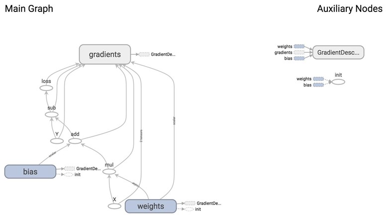
From the graph, you can see that the giant node GradientDescentOptimizer depends on 3 nodes: weights, bias, and gradients (which are automatically taken care of for us).
GradientDescentOptimizer means that our update rule is gradient descent. TensorFlow does auto differentiation for us, then update the values of w and b to minimize the loss. Autodiff is amazing!
By default, the optimizer trains all the trainable variables its objective function depends on. If there are variables that you do not want to train, you can set the keyword trainable=False when you declare a variable. One example of a variable you don''t want to train is the variable global_step, a common variable you will see in many TensorFlow model to keep track of how many times you''ve run your model.
global_step = tf.Variable(0, trainable=False, dtype=tf.int32)
learning_rate = 0.01 * 0.99 ** tf.cast(global_step, tf.float32)
increment_step = global_step.assign_add(1)
optimizer = tf.train.GradientDescentOptimizer(learning_rate) # learning rate can be a tensor
tf.Variable(
initial_value=None,
trainable=True,
collections=None,
validate_shape=True,
caching_device=None,
name=None,
variable_def=None,
dtype=None,
expected_shape=None,
import_scope=None,
constraint=None
)
tf.get_variable(
name,
shape=None,
dtype=None,
initializer=None,
regularizer=None,
trainable=True,
collections=None,
caching_device=None,
partitioner=None,
validate_shape=True,
use_resource=None,
custom_getter=None,
constraint=None
)
You can also ask your optimizer to take gradients of specific variables. You can also modify the gradients calculated by your optimizer.
# create an optimizer.
optimizer = tf.train.GradientDescentOptimizer(learning_rate=0.1)
# compute the gradients for a list of variables.
grads_and_vars = optimizer.compute_gradients(loss, <list of variables>)
# grads_and_vars is a list of tuples (gradient, variable). Do whatever you
# need to the ''gradient'' part, for example, subtract each of them by 1.
subtracted_grads_and_vars = [(gv[0] - 1.0, gv[1]) for gv in grads_and_vars]
# ask the optimizer to apply the subtracted gradients.
optimizer.apply_gradients(subtracted_grads_and_vars)
You can also prevent certain tensors from contributing to the calculation of the derivatives with respect to a specific loss with tf.stop_gradient.
stop_gradient( input, name=None )
This is very useful in situations when you want to freeze certain variables during training. Here are some examples given by TensorFlow''s official documentation.
- When you train a GAN (Generative Adversarial Network) where no backprop should happen through the adversarial example generation process.
- The EM algorithm where the M-step should not involve backpropagation through the output of the E-step.
The optimizer classes automatically compute derivatives on your graph, but you can explicitly ask TensorFlow to calculate certain gradients with tf.gradients.
tf.gradients(
ys,
xs,
grad_ys=None,
name=''gradients'',
colocate_gradients_with_ops=False,
gate_gradients=False,
aggregation_method=None,
stop_gradients=None
)
This method constructs symbolic partial derivatives of sum of ys w.r.t. x in xs. ys and xs are each a Tensor or a list of tensors. grad_ys is a list of Tensor, holding the gradients received by the ys. The list must be the same length as ys.
Technical detail: This is especially useful when training only parts of a model. For example, we can use tf.gradients() to take the derivative G of the loss w.r.t. to the middle layer. Then we use an optimizer to minimize the difference between the middle layer output M and M + G. This only updates the lower half of the network.
List of optimizers
GradientDescentOptimizer is not the only update rule that TensorFlow supports. Here is the list of optimizers that TensorFlow supports, as of 1/17/2017. The names are self-explanatory. You can visit the official documentation for more details:
tf.train.Optimizer
tf.train.GradientDescentOptimizer
tf.train.AdadeltaOptimizer
tf.train.AdagradOptimizer
tf.train.AdagradDAOptimizer
tf.train.MomentumOptimizer
tf.train.AdamOptimizer
tf.train.FtrlOptimizer
tf.train.ProximalGradientDescentOptimizer
tf.train.ProximalAdagradOptimizer
tf.train.RMSPropOptimizer
Sebastian Ruder, a PhD candidate at the Insight Research Centre for Data Analytics did a pretty great comparison of these optimizers in his blog post. If you''re too lazy to read, here is the conclusion:
"RMSprop is an extension of Adagrad that deals with its radically diminishing learning rates. It is identical to Adadelta, except that Adadelta uses the RMS of parameter updates in the numerator update rule. Adam, finally, adds bias-correction and momentum to RMSprop. Insofar, RMSprop, Adadelta, and Adam are very similar algorithms that do well in similar circumstances. Kingma et al. [15] show that its bias-correction helps Adam slightly outperform RMSprop towards the end of optimization as gradients become sparser. Insofar, Adam might be the best overall choice."
TL;DR: Use AdamOptimizer.
Discussion questions
What are some of the real world problems that we can solve using linear regression? Can you write a quick program to do so?
Logistic Regression with MNIST
Let''s build a logistic regression model in TensorFlow solving the good old classifier on the MNIST database.
The MNIST (Mixed National Institute of Standards and Technology database) is one of the most popular databases used for training various image processing systems. It is a database of handwritten digits. The images look like this:
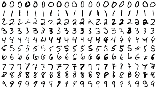
Each image is 28 x 28 pixels. You can flatten each image to be a 1-d tensor of size 784. Each comes with a label from 0 to 9. For example, images on the first row is labelled as 0, the second as 1, and so on. The dataset is hosted on Yann Lecun''s website.
TF Learn (the simplified interface of TensorFlow) has a script that lets you load the MNIST dataset from Yann Lecun''s website and divide it into train set, validation set, and test set.
from tensorflow.examples.tutorials.mnist import input_data
mnist = input_data.read_data_sets(''data/mnist'', one_hot=True)
One-hot encoding
In digital circuits, one-hot refers to a group of bits among which the legal combinations of values are only those with a single high (1) bit and all the others low (0).
In this case, one-hot encoding means that if the output of the image is the digit 7, then the output will be encoded as a vector of 10 elements with all elements being 0, except for the element at index 7 which is 1.
input_data.read_data_sets(''data/mnist'', one_hot=True) returns an instance of learn.datasets.base.Datasets, which contains three generators to 55,000 data points of training data (mnist.train), 10,000 points of test data (mnist.test), and 5,000 points of validation data (mnist.validation). You get the samples of these datasets by calling next_batch(batch_size), for example, mnist.train.next_batch(batch_size) with a batch_size of your choice. However, in real life, we often don''t have access to an off the shelf data parser I thought it''d be nice for us to just read in the MNIST data ourselves. It''s also a good practice because in your real life work, you''re likely to have to write your own data parser.
I''ve already written the code for downloading and parsing MNIST data into numpy arrays in the file utils.py. All you need to do in your program is:
mnist_folder = ''data/mnist''
utils.download_mnist(mnist_folder)
train, val, test = utils.read_mnist(mnist_folder, flatten=True)
We choose flatten=True because we want each image to be flattened into a 1-d tensor. Each of train, val, and test in this case is a tuple of NumPy arrays, the first is a NumPy array of images, the second of labels. We need to create two Dataset objects, one for train set and one for test set (in this example, we won''t be using val set).
train_data = tf.data.Dataset.from_tensor_slices(train)
# train_data = train_data.shuffle(10000) # if you want to shuffle your data
test_data = tf.data.Dataset.from_tensor_slices(test)
The construction of the logistic regression model is pretty similar to the linear regression model. However, now we have A LOT more data. If we calculate gradient after every single data point it''d be painfully slow. Fortunately, we can process the data in batches.
train_data = train_data.batch(batch_size)
test_data = test_data.batch(batch_size)
The next step is to create an iterator to get samples from the two datasets. In the linear regression example, we used only the train set, so it was okay to create an iterator for that dataset and just draw samples from that dataset. When we have more than one dataset, if we have one iterator for each dataset, we would need to build one graph for each iterator! A better way to do it is to create one single iterator and initialize it with a dataset when we need to draw data from that dataset.
iterator = tf.data.Iterator.from_structure(train_data.output_types,
train_data.output_shapes)
img, label = iterator.get_next()
train_init = iterator.make_initializer(train_data) # initializer for train_data
test_init = iterator.make_initializer(test_data) # initializer for test_data
with tf.Session() as sess:
...
for i in range(n_epochs): # train the model n_epochs times
sess.run(train_init) # drawing samples from train_data
try:
while True:
_, l = sess.run([optimizer, loss])
except tf.errors.OutOfRangeError:
pass
# test the model
sess.run(test_init) # drawing samples from test_data
try:
while True:
sess.run(accuracy)
except tf.errors.OutOfRangeError:
pass
Similar to linear regression, you can download the starter file examples/03_logreg_starter.py from the class''s GitHub repo and give it a shot. You can see the solution at examples/03_logreg.py.
Running on my Mac, the batch version of the model with batch size 128 runs in 1 second, while the non-batch model runs in 30 seconds! Note that larger batch size typically requires more epochs since it does fewer update steps. See "mini-batch size" in Bengio''s practical tips. Larger batch size also requires more memory.
We achieved the accuracy of 91.34% after 30 epochs. This is about as good as we can get from a linear classifier.
Shuffling can affect performance: without shuffling, the accuracy is consistently at 91.34%. With shuffle, the accuracy fluctuates between 88% to 93%.
Let''s see what our graph looks like on TensorBoard.
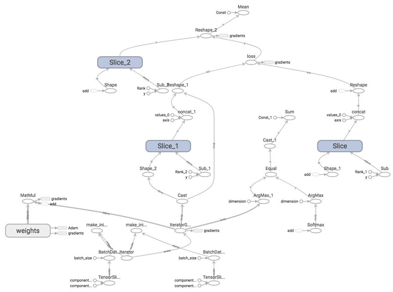
WOW
I know. That''s why we''ll learn how to structure our model in the next lecture!

linear regression and logistic regression with pytorch

import torch
import torch.nn.functional as F
from torch.autograd import variable
x = Variable(torch.Tensor([1]), requires_grad = True)
w = Variable(torch.Tensor([2]), requires_grad = True)
b = Variable(torch.Tensor([3]), requires_grad = True)
requires_grad = False(default) 默认是不对其求梯度的,除非声明为 True
y = w * x + b
# y = 2 * 1 + 3
y.backward()
y.backward 就是自动求导
print(x.grad)
print(w.grad)
print(b.grad)
Variable containing:
 2
[torch.FloatTensor of size 1]

Variable containing:
 1
[torch.FloatTensor of size 1]

Variable containing:
 1
[torch.FloatTensor of size 1]
x = Variable(torch.Tensor([0]), requires_grad = True)
w = Variable(torch.Tensor([2]), requires_grad = True)
b = Variable(torch.Tensor([5]), requires_grad = True)
y = w*x*x + b
y.backward(torch.FloatTensor([1]))
print(x.grad)
Variable containing:
 0
[torch.FloatTensor of size 1]
x = Variable(torch.randn(3), requires_grad = True)
print(x)
Variable containing:
-0.9882
-1.1375
-0.4344
[torch.FloatTensor of size 3]
y = 2*x
y.backward(torch.FloatTensor([1,1,1]))
print(x.grad)
Variable containing:
 2
 2
 2
[torch.FloatTensor of size 3]
grad can be implicitly created only for scalar outputs you have to explicitly write torch.FloatTensor([1,1,1])
y.backward(torch.FloatTensor([0.1, 0.2, 0.3]))
print(x.grad)
Variable containing:
 2.2000
 2.4000
 2.6000
[torch.FloatTensor of size 3]
gradient will accumulate somehow
two ways of saving a model
- save both the model and the parameters
torch.save(model, ''./model.poth'')
- save only the parameters (save the state of the model)
torch.save(model.state_dict(), ''./model_state.pth'')
two ways of loading a model
- load both model and parameters load_model = torch.load(''model.pth'')
- load only parameters ????
import matplotlib.pyplot as plt
import numpy as np
x_train = np.array([[3.3], [4.4], [5.5], [6.71], [6.93], [4.168],
                    [9.779], [6.182], [7.59], [2.167], [7.042],
                    [10.791], [5.313], [7.997], [3.1]], dtype=np.float32)

y_train = np.array([[1.7], [2.76], [2.09], [3.19], [1.694], [1.573],
                    [3.366], [2.596], [2.53], [1.221], [2.827],
                    [3.465], [1.65], [2.904], [1.3]], dtype=np.float32)
plt.scatter(x_train, y_train, )
<matplotlib.collections.PathCollection at 0x10b695f28>

#首先把numpyarray类型的数据转换成torch.tensor,使用torch.from_numpy方法
x_train = torch.from_numpy(x_train)
y_train = torch.from_numpy(y_train)
class LinearRegression(torch.nn.Module):
    def __init__(self):
        super(LinearRegression, self).__init__()
        self.linear = nn.Linear(1, 1)
        # basicly this is x*w+b=y
    def forward(self, x):
        out = self.linear(x)
        return out
# class LinearRegression(torch.nn.Module):
#     def __init__(self, input_num, hidden_num, output_num):
#         super(LinearRegression, self).__init__()
#         self.linear1 = nn.Linear(input_num, hidden_num)
#         self.linear2 = nn.Linear(hidden_num, output_num)
#         # basicly this is x*w+b=y
#     def forward(self, x):
#         x = F.relu(self.linear1(x))
#         out = (self.linear2(x))
#         return out
if torch.cuda.is_available():
    model = LinearRegression().cuda()
net = LinearRegression()
print(net)
LinearRegression(
  (linear): Linear(in_features=1, out_features=1)
)
criterion = torch.nn.MSELoss()
optimizer = torch.optim.SGD(net.parameters(), lr = 1e-3)
num_epochs = 100
for epoch in range(num_epochs):
    if torch.cuda.is_available():
        inputs = Variable(x_train).cuda()
        target = Variable(y_train).cuda()
    else:
        inputs = Variable(x_train)
        target = Variable(y_train)
    # forward
    out = net(inputs)
    loss = criterion(out, target)
    # backward
    optimizer.zero_grad()
    loss.backward()
    optimizer.step()

    if(epoch + 1) % 20 == 0:
        print(''epoch[{}/{}], loss: {:.6f}''.format(epoch+1, num_epochs, loss.data[0]))
        # loss is a Variable, by calling data, we get the data of the Variable
epoch[20/100], loss: 0.300034
epoch[40/100], loss: 0.298694
epoch[60/100], loss: 0.297367
epoch[80/100], loss: 0.296054
epoch[100/100], loss: 0.294755
net.eval() # evaluate mode
predict = net(Variable(x_train))
predict = predict.data.numpy()
plt.scatter(x_train.numpy(), y_train.numpy())
plt.plot(x_train.numpy(), predict, )
plt.show()

n_data = torch.ones(100, 2)
x0 = torch.normal(2*n_data, 1)      # class0 x data (tensor), shape=(100, 2)
y0 = torch.zeros(100)               # class0 y data (tensor), shape=(100, 1)
x1 = torch.normal(-2*n_data, 1)     # class1 x data (tensor), shape=(100, 2)
y1 = torch.ones(100)                # class1 y data (tensor), shape=(100, 1)
x = torch.cat((x0, x1), 0).type(torch.FloatTensor)  # shape (200, 2) FloatTensor = 32-bit floating
# print(x.numpy().shape)
y = torch.cat((y0, y1), ).type(torch.LongTensor)    # shape (200,) LongTensor = 64-bit integer
plt.scatter(x.numpy()[:,0], x.numpy()[:,1], c = y)
<matplotlib.collections.PathCollection at 0x10d1b4dd8>

class LogisticRegression(torch.nn.Module):
    def __init__(self, input_num, hidden_num, output_num):
        super(LogisticRegression, self).__init__()
        self.hidden = torch.nn.Linear(input_num, hidden_num)
        self.output = torch.nn.Linear(hidden_num, output_num)

    def forward(self, x):
        x = torch.nn.functional.relu(self.hidden(x))
        out = self.output(x)
        return x
net = LogisticRegression(2, 10, 2)
print(net)
LogisticRegression(
  (hidden): Linear(in_features=2, out_features=10)
  (output): Linear(in_features=10, out_features=2)
)
criterion = torch.nn.CrossEntropyLoss()
optimizer = torch.optim.SGD(net.parameters(), lr = 1e-1)
if torch.cuda.is_available():
    inputx = Variable(x).cuda()
    targety = Variable(y).cuda()
else:
    inputx = Variable(x)
    targety = Variable(y)
num_epochs = 1000
for epoch in range(num_epochs):
    # forward
    out = net(inputx)
    loss = criterion(out, targety)
    # backward
    optimizer.zero_grad()
    loss.backward()
    optimizer.step()

    if epoch % 40 == 0:
        print(''Epoch[{}/{}], loss: {:.6f}''.format(epoch, num_epochs, loss.data[0]))
#     if epoch % 20 == 0:
# plot and show learning process
plt.cla()
prediction = torch.max(out, 1)[1]
# print(prediction.data.numpy().shape)
pred_y = prediction.data.numpy().squeeze()
# print(pred_y.shape)
target_y = y.numpy()
plt.scatter(x.numpy()[:, 0], x.numpy()[:, 1], c=pred_y, s=100, lw=0, cmap=''RdYlGn'')
accuracy = sum(pred_y == target_y)/200.
plt.text(1.5, -4, ''Accuracy=%.2f'' % accuracy, fontdict={''size'': 20, ''color'':  ''red''})
#         plt.pause(0.1)

# plt.ioff()
plt.show()
Epoch[0/1000], loss: 3.279978
Epoch[40/1000], loss: 0.165580
Epoch[80/1000], loss: 0.085501
Epoch[120/1000], loss: 0.059977
Epoch[160/1000], loss: 0.047022
Epoch[200/1000], loss: 0.039068
Epoch[240/1000], loss: 0.033637
Epoch[280/1000], loss: 0.029672
Epoch[320/1000], loss: 0.026636
Epoch[360/1000], loss: 0.024226
Epoch[400/1000], loss: 0.022261
Epoch[440/1000], loss: 0.020624
Epoch[480/1000], loss: 0.019237
Epoch[520/1000], loss: 0.018045
Epoch[560/1000], loss: 0.017008
Epoch[600/1000], loss: 0.016096
Epoch[640/1000], loss: 0.015287
Epoch[680/1000], loss: 0.014565
Epoch[720/1000], loss: 0.013916
Epoch[760/1000], loss: 0.013329
Epoch[800/1000], loss: 0.012795
Epoch[840/1000], loss: 0.012310
Epoch[880/1000], loss: 0.011866
Epoch[920/1000], loss: 0.011458
Epoch[960/1000], loss: 0.011080

net.eval()
xx = np.linspace(-4,4,10000).reshape(10000, 1)
yy = 4*np.sin(xx*100).reshape(10000, 1)
xy = np.concatenate((xx, yy), axis = 1)
xy = torch.from_numpy(xy).type(torch.FloatTensor)
xy = Variable(xy)
pred = net(xy)
# print(pred.data.numpy().shape)
# print(pred[:6, :])
pred = torch.max(pred, 1)[1]
# print(len(pred))

# print(len(pred))
# print(pred.data.numpy().shape)
# print(pred[:6])
pred = pred.data.numpy().squeeze()
plt.scatter(xy.data.numpy()[:, 0], xy.data.numpy()[:, 1], c = pred, s = 100, lw = 0, cmap = ''RdYlGn'')
plt.show()

我们今天的关于用于LogisticRegression的Spark MLLib TFIDF实现和logisticregression python的分享已经告一段落,感谢您的关注,如果您想了解更多关于2017年2月14日 Logistic Regression、GridSearchCV的LogisticRegression无法收敛、Linear and Logistic Regression in TensorFlow、linear regression and logistic regression with pytorch的相关信息,请在本站查询。
本文标签:


