这篇文章主要围绕pythonpandas时间序列图,如何在ts.plot和之外设置xlim和xticks?展开,旨在为您提供一份详细的参考资料。我们将全面介绍pythonpandas时间序列图,如何在
这篇文章主要围绕python pandas时间序列图,如何在ts.plot和之外设置xlim和xticks?展开,旨在为您提供一份详细的参考资料。我们将全面介绍python pandas时间序列图,如何在ts.plot的优缺点,解答之外设置xlim和xticks?的相关问题,同时也会为您带来pandas小记:pandas时间序列分析和处理Timeseries、pandas时间序列之pd.to_datetime()的实现、pandas时间序列之如何将int转换成datetime格式、Pandas时间序列和分组聚合的实用方法。
本文目录一览:- python pandas时间序列图,如何在ts.plot()之外设置xlim和xticks?(pandas时间序列处理)
- pandas小记:pandas时间序列分析和处理Timeseries
- pandas时间序列之pd.to_datetime()的实现
- pandas时间序列之如何将int转换成datetime格式
- Pandas时间序列和分组聚合
之外设置xlim和xticks?(pandas时间序列处理)")
python pandas时间序列图,如何在ts.plot()之外设置xlim和xticks?(pandas时间序列处理)
fig = plt.figure()
ax = fig.gca()
ts.plot(ax=ax)
我知道我可以在熊猫绘图例程ts.plot(xlim = …)中设置xlim,但是在熊猫绘图完成后如何更改它?
ax.set_xlim(( t0.toordinal(),t1.toordinal() )
有时可以正常工作,但是如果熊猫将xaxis格式化为距时代数月而不是几天,那么这将很难失败。
无论如何,我们是否知道熊猫如何将日期转换为xaxis,然后以相同的方式转换我的xlim?
谢谢。

pandas小记:pandas时间序列分析和处理Timeseries
http://blog.csdn.net/pipisorry/article/details/52209377
pandas 最基本的时间序列类型就是以时间戳(TimeStamp)为 index 元素的 Series 类型。
其它时间序列处理相关的包
[P4J 0.6: Periodic light curve analysis tools based on Information Theory]
[p4j github]
pandas时序数据文件读取
dateparse = lambda dates: pd.datetime.strptime(dates, ''%Y-%m'')
data = pd.read_csv(''AirPassengers.csv'', parse_dates=''Month'', index_col=''Month'',date_parser=dateparse)
print data.head()
read_csv时序参数
parse_dates:这是指定含有时间数据信息的列。正如上面所说的,列的名称为“月份”。
index_col:使用pandas 的时间序列数据背后的关键思想是:目录成为描述时间数据信息的变量。所以该参数告诉pandas使用“月份”的列作为索引。
date_parser:指定将输入的字符串转换为可变的时间数据。Pandas默认的数据读取格式是‘YYYY-MM-DD HH:MM:SS’?如需要读取的数据没有默认的格式,就要人工定义。这和dataparse的功能部分相似,这里的定义可以为这一目的服务。The default uses dateutil.parser.parser to do the conversion.
[pandas.read_csv]
[python模块:时间处理模块]
时间序列分析和处理Time Series
pandas has simple, powerful, and efficient functionality for performingresampling operations during frequency conversion (e.g., converting secondlydata into 5-minutely data). This is extremely common in, but not limited to,financial applications.
时序数据生成和表示
c = pandas.Timestamp(''2012-01-01 00:00:08'')
In [103]: rng = pd.date_range(''1/1/2012'', periods=100, freq=''S'')

In [104]: ts = pd.Series(np.random.randint(0, 500, len(rng)), index=rng)

In [105]: ts.resample(''5Min'', how=''sum'')
Out[105]:
2012-01-01    25083
Freq: 5T, dtype: int32
Time zone representation
In [106]: rng = pd.date_range(''3/6/2012 00:00'', periods=5, freq=''D'')

In [107]: ts = pd.Series(np.random.randn(len(rng)), rng)

In [108]: ts
Out[108]:
2012-03-06    0.464000
2012-03-07    0.227371
2012-03-08   -0.496922
2012-03-09    0.306389
2012-03-10   -2.290613
Freq: D, dtype: float64

In [109]: ts_utc = ts.tz_localize(''UTC'')

In [110]: ts_utc
Out[110]:
2012-03-06 00:00:00+00:00    0.464000
2012-03-07 00:00:00+00:00    0.227371
2012-03-08 00:00:00+00:00   -0.496922
2012-03-09 00:00:00+00:00    0.306389
2012-03-10 00:00:00+00:00   -2.290613
Freq: D, dtype: float64
时序转换
Convert to another time zone
In [111]: ts_utc.tz_convert(''US/Eastern'')
Out[111]:
2012-03-05 19:00:00-05:00    0.464000
2012-03-06 19:00:00-05:00    0.227371
2012-03-07 19:00:00-05:00   -0.496922
2012-03-08 19:00:00-05:00    0.306389
2012-03-09 19:00:00-05:00   -2.290613
Freq: D, dtype: float64
Converting between time span representations
In [112]: rng = pd.date_range(''1/1/2012'', periods=5, freq=''M'')
In [113]: ts = pd.Series(np.random.randn(len(rng)), index=rng)
In [114]: ts
Out[114]:
2012-01-31   -1.134623
2012-02-29   -1.561819
2012-03-31   -0.260838
2012-04-30    0.281957
2012-05-31    1.523962
Freq: M, dtype: float64

In [115]: ps = ts.to_period()
In [116]: ps
Out[116]:
2012-01   -1.134623
2012-02   -1.561819
2012-03   -0.260838
2012-04    0.281957
2012-05    1.523962
Freq: M, dtype: float64

In [117]: ps.to_timestamp()
Out[117]:
2012-01-01   -1.134623
2012-02-01   -1.561819
2012-03-01   -0.260838
2012-04-01    0.281957
2012-05-01    1.523962
Freq: MS, dtype: float64
Converting between period and timestamp enables some convenient arithmeticfunctions to be used. In the following example, we convert a quarterlyfrequency with year ending in November to 9am of the end of the month followingthe quarter end:
In [118]: prng = pd.period_range(''1990Q1'', ''2000Q4'', freq=''Q-NOV'')
In [119]: ts = pd.Series(np.random.randn(len(prng)), prng)
In [120]: ts.index = (prng.asfreq(''M'', ''e'') + 1).asfreq(''H'', ''s'') + 9
In [121]: ts.head()
Out[121]:
1990-03-01 09:00   -0.902937
1990-06-01 09:00    0.068159
1990-09-01 09:00   -0.057873
1990-12-01 09:00   -0.368204
1991-03-01 09:00   -1.144073
Freq: H, dtype: float64
[pandas-docs/stable/timeseries]
[pandas cookbook Timeseries]
时序处理相关函数
pandas.to_datetime(*args, **kwargs)
Convert argument to datetime.
lz觉得此函数一般是对不明确类型进行转换,如果直接对datetime类型转换太慢不值得,有其它方法。
Series.dt.normalize(*args, **kwargs)
Return DatetimeIndex with times to midnight. Length is unaltered.直接调用应该就是只取datetime的date部分,即重置time部分,而保持datetime类型不变。
DatetimeIndex.normalize()
Return DatetimeIndex with times to midnight. Length is unaltered
DatetimeIndex相关的函数
Note: pandas时间序列series的index必须是DatetimeIndex不能是Index,也就是如果index是从dataframe列中转换来的,其类型必须是datetime类型,不能是date、object等等其它类型!否则在很多处理包中会报错。
ts.index
返回DatetimeIndex([''2015-07-02'', ''2015-07-03'', ''2015-07-04'', ''2015-07-05'', ... ''2016-10-26'', ''2016-10-27'', ''2016-10-28'', ''2016-10-29''],
dtype=''datetime64[ns]'', name=''time'', length=481, freq=None)
freq也可以通过ts.index.inferred_freq查看
series对象的dt存取器 .dt accessor
Series.dt()
Accessor object for datetimelike properties of the Series values.
示例
s.dt.date
>>> s.dt.hour
>>> s.dt.second
>>> s.dt.quarter
Returns a Series indexed like the original Series. Raises TypeError if the Series does not contain datetimelike values.
Series datetime类型处理
示例:将series中datetime类型只保留date部分而不改变数据类型,即数据类型仍为datetime
s.map(pd.Timestamp.date) 或者 s.map(lambda x: pd.to_datetime(x.date()))
但是pd.Timestamp.date会将数据的类型从datetime类型转换成date类型,在pd中显示是object类型;而转换成datetime的函数pd.to_datetime特别慢而耗时。
一个最好的转换方式是直接进行类型转换
Converting to datetime64[D]:df.dates.values.astype(''M8[D]'') Though re-assigning that to a DataFrame col will revert it back to [ns].
所以可以这样实现user_pay_df[''time''] = user_pay_df[''time''].dt.date.astype(''M8[D]'')或者user_pay_df[''time''] = user_pay_df[''time''].dt.date.astype(np.datetime64)
不过这仍不是最快的方法,lz找到一个更快的方法
重置datetime的time部分
user_pay_df[''time''] = user_pay_df[''time''].dt.normalize()[Keep only date part when using pandas.to_datetime]
uid sid time
0 22127870 1862 2015-12-25 17:00:00
1 3434231 1862 2016-10-05 11:00:00
2 16955285 1862 2016-02-10 15:00:00
uid int64
sid int64
time datetime64[ns]
dtype: object
uid sid time
0 22127870 1862 2015-12-25
1 3434231 1862 2016-10-05
2 16955285 1862 2016-02-10
uid int64
sid int64
time datetime64[ns]
皮皮blog
pandas时序类型
pandas 的 TimeStamp
pandas 最基本的时间日期对象是一个从 Series 派生出来的子类 TimeStamp,这个对象与 datetime 对象保有高度兼容性,可通过 pd.to_datetime() 函数转换。(一般是从 datetime 转换为 Timestamp)
lang:python
>>> pd.to_datetime(now)
Timestamp(''2014-06-17 15:56:19.313193'', tz=None)
>>> pd.to_datetime(np.nan)
NaT
pandas 的时间序列
pandas 最基本的时间序列类型就是以时间戳(TimeStamp)为 index 元素的 Series 类型。
lang:python
>>> dates = [datetime(2011,1,1),datetime(2011,1,2),datetime(2011,1,3)]
>>> ts = Series(np.random.randn(3),index=dates)
>>> ts
2011-01-01    0.362289
2011-01-02    0.586695
2011-01-03   -0.154522
dtype: float64
>>> type(ts)
<class ''pandas.core.series.Series''>
>>> ts.index
<class ''pandas.tseries.index.DatetimeIndex''>
[2011-01-01, ..., 2011-01-03]
Length: 3, Freq: None, Timezone: None
>>> ts.index[0]
Timestamp(''2011-01-01 00:00:00'', tz=None)
时间序列之间的算术运算会自动按时间对齐。
时间序列的索引、选取、子集构造
时间序列只是 index 比较特殊的 Series ,因此一般的索引操作对时间序列依然有效。其特别之处在于对时间序列索引的操作优化。
先在序列对象选择一个特殊值。可以通过以下两种方式实现:
1 使用各种字符串进行索引:
lang:python
>>> ts[''20110101'']
0.36228897878097266
>>> ts[''2011-01-01'']
0.36228897878097266
>>> ts[''01/01/2011'']
0.36228897878097266
2 Import the datetime library and use ''datetime'' function:
from datetime import datetime
ts[datetime(1949,1,1)]对于较长的序列,还可以只传入 “年” 或 “年月” 选取切片:
>>> ts
2011-01-01    0.362289
2011-01-02    0.586695
2011-01-03   -0.154522
2012-12-25    0.111869
dtype: float64
>>> ts[''2012'']
2012-12-25    0.111869
dtype: float64
>>> ts[''2011-1-2'':''2012-12'']
2011-01-02    0.586695
2011-01-03   -0.154522
2012-12-25    0.111869
dtype: float64
4 除了这种字符串切片方式外,还有一种实例方法可用:ts.truncate(after=''2011-01-03'')。
值得注意的是,切片时使用的字符串时间戳并不必存在于 index 之中,如 ts.truncate(before=''3055'') 也是合法的。
Time/Date Components
There are several time/date properties that one can access from Timestamp or a collection of timestamps like a DateTimeIndex.
| Property | Description |
|---|---|
| year | The year of the datetime |
| month | The month of the datetime |
| day | The days of the datetime |
| hour | The hour of the datetime |
| minute | The minutes of the datetime |
| second | The seconds of the datetime |
| microsecond | The microseconds of the datetime |
| nanosecond | The nanoseconds of the datetime |
| date | Returns datetime.date |
| time | Returns datetime.time |
| dayofyear | The ordinal day of year |
| weekofyear | The week ordinal of the year |
| week | The week ordinal of the year |
| dayofweek | The numer of the day of the week with Monday=0, Sunday=6 |
| weekday | The number of the day of the week with Monday=0, Sunday=6 |
| weekday_name | The name of the day in a week (ex: Friday) |
| quarter | Quarter of the date: Jan=Mar = 1, Apr-Jun = 2, etc. |
| days_in_month | The number of days in the month of the datetime |
| is_month_start | Logical indicating if first day of month (defined by frequency) |
| is_month_end | Logical indicating if last day of month (defined by frequency) |
| is_quarter_start | Logical indicating if first day of quarter (defined by frequency) |
| is_quarter_end | Logical indicating if last day of quarter (defined by frequency) |
| is_year_start | Logical indicating if first day of year (defined by frequency) |
| is_year_end | Logical indicating if last day of year (defined by frequency) |
Furthermore, if you have a Series with datetimelike values, then you can access these properties via the .dt accessor, see the docs.
[Time/Date Components¶]
日期的范围、频率以及移动
pandas 中的时间序列一般被默认为不规则的,即没有固定的频率。但出于分析的需要,我们可以通过插值的方式将序列转换为具有固定频率的格式。一种快捷方式是使用 .resample(rule) 方法:
lang:python
>>> ts
2011-01-01    0.362289
2011-01-02    0.586695
2011-01-03   -0.154522
2011-01-06    0.222958
dtype: float64
>>> ts.resample(''D'')
2011-01-01    0.362289
2011-01-02    0.586695
2011-01-03   -0.154522
2011-01-04         NaN
2011-01-05         NaN
2011-01-06    0.222958
Freq: D, dtype: float64
生成日期范围
pd.date_range() 可用于生成指定长度的 DatetimeIndex。参数可以是起始结束日期,或单给一个日期,加一个时间段参数。日期是包含的。
lang:python
>>> pd.date_range(''20100101'',''20100110'')
<class ''pandas.tseries.index.DatetimeIndex''>
[2010-01-01, ..., 2010-01-10]
Length: 10, Freq: D, Timezone: None
>>> pd.date_range(start=''20100101'',periods=10)
<class ''pandas.tseries.index.DatetimeIndex''>
[2010-01-01, ..., 2010-01-10]
Length: 10, Freq: D, Timezone: None
>>> pd.date_range(end=''20100110'',periods=10)
<class ''pandas.tseries.index.DatetimeIndex''>
[2010-01-01, ..., 2010-01-10]
Length: 10, Freq: D, Timezone: None
默认情况下,date_range 会按天计算时间点。这可以通过 freq 参数进行更改,如 “BM” 代表 bussiness end of month。
lang:python
>>> pd.date_range(''20100101'',''20100601'',freq=''BM'')
<class ''pandas.tseries.index.DatetimeIndex''>
[2010-01-29, ..., 2010-05-31]
Length: 5, Freq: BM, Timezone: None
频率和日期偏移量
pandas 中的频率是由一个基础频率和一个乘数组成的。基础频率通常以一个字符串别名表示,如上例中的 “BM”。对于每个基础频率,都有一个被称为日期偏移量(date offset)的对象与之对应。可以通过实例化日期偏移量来创建某种频率:
lang:python
>>> Hour()
<Hour>
>>> Hour(2)
<2 * Hours>
>>> Hour(1) + Minute(30)
<90 * Minutes>
但一般来说不必这么麻烦,使用前面提过的字符串别名来创建频率就可以了:
lang:python
>>> pd.date_range(''00:00'',''12:00'',freq=''1h20min'')
<class ''pandas.tseries.index.DatetimeIndex''>
[2014-06-17 00:00:00, ..., 2014-06-17 12:00:00]
Length: 10, Freq: 80T, Timezone: None
可用的别名,可以通过 help() 或 文档来查询,这里就不写了。
移动(超前和滞后)数据
移动(shifting)指的是沿着时间轴将数据前移或后移。Series 和 DataFrame 都有一个 .shift() 方法用于执行单纯的移动操作,index 维持不变:
lang:python
>>> ts
2011-01-01    0.362289
2011-01-02    0.586695
2011-01-03   -0.154522
2011-01-06    0.222958
dtype: float64
>>> ts.shift(2)
2011-01-01         NaN
2011-01-02         NaN
2011-01-03    0.362289
2011-01-06    0.586695
dtype: float64
>>> ts.shift(-2)
2011-01-01   -0.154522
2011-01-02    0.222958
2011-01-03         NaN
2011-01-06         NaN
dtype: float64
上例中因为移动操作产生了 NA 值,另一种移动方法是移动 index,而保持数据不变。这种移动方法需要额外提供一个 freq 参数来指定移动的频率:
lang:python
>>> ts.shift(2,freq=''D'')
2011-01-03    0.362289
2011-01-04    0.586695
2011-01-05   -0.154522
2011-01-08    0.222958
dtype: float64
>>> ts.shift(2,freq=''3D'')
2011-01-07    0.362289
2011-01-08    0.586695
2011-01-09   -0.154522
2011-01-12    0.222958
dtype: float64
时期及其算术运算
本节使用的时期(period)概念不同于前面的时间戳(timestamp),指的是一个时间段。但在使用上并没有太多不同,pd.Period 类的构造函数仍需要一个时间戳,以及一个 freq 参数。freq 用于指明该 period 的长度,时间戳则说明该 period 在公园时间轴上的位置。
lang:python
>>> p = pd.Period(2010,freq=''M'')
>>> p
Period(''2010-01'', ''M'')
>>> p + 2
Period(''2010-03'', ''M'')
上例中我给 period 的构造器传了一个 “年” 单位的时间戳和一个 “Month” 的 freq,pandas 便自动把 2010 解释为了 2010-01。
period_range 函数可用于创建规则的时间范围:
lang:python
>>> pd.period_range(''2010-01'',''2010-05'',freq=''M'')
<class ''pandas.tseries.period.PeriodIndex''>
freq: M
[2010-01, ..., 2010-05]
length: 5
PeriodIndex 类保存了一组 period,它可以在任何 pandas 数据结构中被用作轴索引:
lang:python
>>> Series(np.random.randn(5),index=pd.period_range(''201001'',''201005'',freq=''M''))
2010-01    0.755961
2010-02   -1.074492
2010-03   -0.379719
2010-04    0.153662
2010-05   -0.291157
Freq: M, dtype: float64
时期的频率转换
Period 和 PeriodIndex 对象都可以通过其 .asfreq(freq, method=None, how=None) 方法被转换成别的频率。
lang:python
>>> p = pd.Period(''2007'',freq=''A-DEC'')
>>> p.asfreq(''M'',how=''start'')
Period(''2007-01'', ''M'')
>>> p.asfreq(''M'',how=''end'')
Period(''2007-12'', ''M'')
>>> ts = Series(np.random.randn(1),index=[p])
>>> ts
2007   -0.112347
Freq: A-DEC, dtype: float64
>>> ts.asfreq(''M'',how=''start'')
2007-01   -0.112347
Freq: M, dtype: float64
时间戳与时期间相互转换
以时间戳和以时期为 index 的 Series 和 DataFrame 都有一对 .to_period() 和 to_timestamp(how=''start'') 方法用于互相转换 index 的类型。因为从 period 到 timestamp 的转换涉及到一个取端值的问题,所以需要一个额外的 how 参数,默认为 ''start'':
lang:python
>>> ts = Series(np.random.randn(5),index=pd.period_range(''201001'',''201005'',freq=''M''))
>>> ts
2010-01   -0.312160
2010-02    0.962652
2010-03   -0.959478
2010-04    1.240236
2010-05   -0.916218
Freq: M, dtype: float64
>>> ts.to_timestamp()
2010-01-01   -0.312160
2010-02-01    0.962652
2010-03-01   -0.959478
2010-04-01    1.240236
2010-05-01   -0.916218
Freq: MS, dtype: float64
>>> ts.to_timestamp(how=''end'')
2010-01-31   -0.312160
2010-02-28    0.962652
2010-03-31   -0.959478
2010-04-30    1.240236
2010-05-31   -0.916218
Freq: M, dtype: float64
>>> ts.to_timestamp().to_period()
2010-01-01 00:00:00.000   -0.312160
2010-02-01 00:00:00.000    0.962652
2010-03-01 00:00:00.000   -0.959478
2010-04-01 00:00:00.000    1.240236
2010-05-01 00:00:00.000   -0.916218
Freq: L, dtype: float64
>>> ts.to_timestamp().to_period(''M'')
2010-01   -0.312160
2010-02    0.962652
2010-03   -0.959478
2010-04    1.240236
2010-05   -0.916218
Freq: M, dtype: float64
重采样及频率转换
重采样(resampling)指的是将时间序列从一个频率转换到另一个频率的过程。pandas 对象都含有一个.resample(freq, how=None, axis=0, fill_method=None, closed=None, label=None, convention=''start'', kind=None, loffset=None, limit=None, base=0) 方法用于实现这个过程。
本篇最前面曾用 resample 规整化过时间序列。当时进行的是插值操作,因为原索引的频率与给出的 freq 参数相同。resample 方法更多的应用场合是 freq 发生改变的时候,这时操作就分为升采样(upsampling)和降采样(downsampling)两种。具体的区别都体现在参数里。
lang:python
>>> ts
2010-01   -0.312160
2010-02    0.962652
2010-03   -0.959478
2010-04    1.240236
2010-05   -0.916218
Freq: M, dtype: float64
>>> ts.resample(''D'',fill_method=''ffill'')#升采样
2010-01-01   -0.31216
2010-01-02   -0.31216
2010-01-03   -0.31216
2010-01-04   -0.31216
2010-01-05   -0.31216
2010-01-06   -0.31216
2010-01-07   -0.31216
2010-01-08   -0.31216
2010-01-09   -0.31216
2010-01-10   -0.31216
2010-01-11   -0.31216
2010-01-12   -0.31216
2010-01-13   -0.31216
2010-01-14   -0.31216
2010-01-15   -0.31216
...
2010-05-17   -0.916218
2010-05-18   -0.916218
2010-05-19   -0.916218
2010-05-20   -0.916218
2010-05-21   -0.916218
2010-05-22   -0.916218
2010-05-23   -0.916218
2010-05-24   -0.916218
2010-05-25   -0.916218
2010-05-26   -0.916218
2010-05-27   -0.916218
2010-05-28   -0.916218
2010-05-29   -0.916218
2010-05-30   -0.916218
2010-05-31   -0.916218
Freq: D, Length: 151
>>> ts.resample(''A-JAN'',how=''sum'')#降采样
2010   -0.312160
2011    0.327191
Freq: A-JAN, dtype: float64
[pandas 时间序列操作]
from: http://blog.csdn.net/pipisorry/article/details/52209377
ref: [时间序列预测全攻略(附带Python代码)]
[概率论:假设检验-t检验和Augmented Dickey–Fuller test ]
[Complete guide to create a Time Series Forecast (with Codes in Python)]
的实现")
pandas时间序列之pd.to_datetime()的实现
解析来自各种来源和格式的时间序列信息
pd.to_datetime(
    arg,#int, float, str, datetime, list, tuple, 1-d array, Series DataFrame/dict-like
    errors=''raise'',# {''ignore'', ''raise'', ''coerce''}, default ''raise''
    dayfirst=False,
    yearfirst=False,
    utc=None,
    format=None,#格式,比如 "%d/%m/%Y"
    exact=True,
    unit=None,#单位str, default ''ns'',可以是(D,s,ms,us,ns)
    infer_datetime_format=False,
    origin=''unix'',#指定从什么时间开始,默认为19700101
    cache=True,
)
时间序列解析之小试牛刀
pd.to_datetime()
import datetime
import pandas as pd
import numpy as np
dti = pd.to_datetime([''1/1/2018'', np.datetime64(''2018-01-01''),
                      datetime.datetime(2018, 1, 1)])
dti
DatetimeIndex([‘2018-01-01’, ‘2018-01-01’, ‘2018-01-01’], dtype=‘datetime64[ns]’, freq=None)
pd.to_datetime([''2020-04-20'', ''20/04/2020'',''Apr 20 2020''])
DatetimeIndex([‘2020-04-20’, ‘2020-04-20’, ‘2020-04-20’], dtype=‘datetime64[ns]’, freq=None)
import time
time.asctime()
‘Tue Apr 7 21:50:17 2020’
pd.to_datetime(time.asctime())
Timestamp(‘2020-04-07 21:50:17’)
还有更加偷懒的办法,假如整理数据时遇到了大量的时间需要输入,比如2020-11-11 00:00:00,输入-和:太浪费时间了,而且时间之间没有什么变化规律可循,这种情况下可以直接输入20201111000000进行记录,之后再借助pd.to_datetime()解析,省时省力一步到位。
pd.to_datetime(''20201111000000'')Timestamp(‘2020-11-11 00:00:00’)
时间序列解析之磨刀霍霍
1. 指定识别的format
pd.to_datetime(''2020/12/12'', format=''%Y/%m/%d'')Timestamp(‘2020-12-12 00:00:00’)
pd.to_datetime(''12-11-2010 00:00'', format=''%d-%m-%Y %H:%M'')Timestamp(‘2010-11-12 00:00:00’)
2. 遇到DataFrame
df = pd.DataFrame({''year'': [2015, 2016],
   ....:                    ''month'': [2, 3],
   ....:                    ''day'': [4, 5],
   ....:                    ''hour'': [2, 3]})
df
year month day hour
0 2015 2 4 2
1 2016 3 5 3
pd.to_datetime(df)
0 2015-02-04 02:00:00
1 2016-03-05 03:00:00
dtype: datetime64[ns]
pd.to_datetime(df[[''year'',''month'',''day'']])
0 2015-02-04
1 2016-03-05
dtype: datetime64[ns]
3. 遇到不能识别的处理方法
pd.to_datetime([''2009/07/31'', ''asd''], errors=''ignore'')
Index([‘2009/07/31’, ‘asd’], dtype=‘object’)
pd.to_datetime([''2009/07/31'', ''asd''], errors=''raise'')
ParserError: Unknown string format: asd
pd.to_datetime([''2009/07/31'', ''asd''], errors=''coerce'')
DatetimeIndex([‘2009-07-31’, ‘NaT’], dtype=‘datetime64[ns]’, freq=None)
4. origin的用法
指定时间
pd.to_datetime([1, 2, 3], unit=''D'', origin=pd.Timestamp(''1960-01-01''))
DatetimeIndex([‘1960-01-02'', ‘1960-01-03'', ‘1960-01-04''], dtype=‘datetime64[ns]'', freq=None)
不指定时间则默认从19700101开始
pd.to_datetime([1, 2, 3], unit=''D'')
DatetimeIndex([‘1970-01-02'', ‘1970-01-03'', ‘1970-01-04''], dtype=‘datetime64[ns]'', freq=None)
到此这篇关于pandas时间序列之pd.to_datetime()的实现的文章就介绍到这了,更多相关pandas pd.to_datetime()内容请搜索以前的文章或继续浏览下面的相关文章希望大家以后多多支持!
- pandas时间序列之如何将int转换成datetime格式
- pandas中的Timestamp只保留日期不显示时间
- pandas实现datetime64与unix时间戳互转
- Pandas处理时间序列数据操作详解
- Pandas中常用的七个时间戳处理函数使用总结
- Pandas 时间序列分析中的resample函数
- Python Pandas高级教程之时间处理
- pandas 时间偏移的实现
- Pandas数据分析固定时间点和时间差

pandas时间序列之如何将int转换成datetime格式
将int转换成datetime格式
原始时间格式
users[''timestamp_first_active''].head()
原始结果:
0 20090319043255
1 20090523174809
2 20090609231247
3 20091031060129
4 20091208061105
Name: timestamp_first_active, dtype: object
错误的转换
pd.to_datetime(sers[''timestamp_first_active''])
错误的结果类似这样:
0 1970-01-01 00:00:00.020201010
1 1970-01-01 00:00:00.020200920
Name: time, dtype: datetime64[ns]
正确的做法
先将int转换成str ,再转成时间:
users[''timestamp_first_active'']=users[''timestamp_first_active''].astype(''str'')
users[''timestamp_first_active'']=pd.to_datetime(users[''timestamp_first_active''])
pandas 时间数据处理
转化时间类型
to_datetime()方法
to_datetime()方法支持将 int, float, str, datetime, list, tuple, 1-d array, Series, DataFrame/dict-like 类型的数据转化为时间类型
import pandas as pd

# str ---> 转化为时间类型:
ret = pd.to_datetime(''2022-3-9'')
print(ret)
print(type(ret))
"""
2022-03-09 00:00:00
<class ''pandas._libs.tslibs.timestamps.Timestamp''>   ---pandas中默认支持的时间点的类型
"""

# 字符串的序列 --->转化成时间类型:
ret = pd.to_datetime([''2022-3-9'', ''2022-3-8'', ''2022-3-7'', ''2022-3-6''])
print(ret)
print(type(ret))
"""
DatetimeIndex([''2022-03-09'', ''2022-03-08'', ''2022-03-07'', ''2022-03-06''], dtype=''datetime64[ns]'', freq=None)
<class ''pandas.core.indexes.datetimes.DatetimeIndex''> ----pandas中默认支持的时间序列的类型
"""
# dtype = ''datetime64[ns]'' ----> numpy中的时间数据类型!
DatetimeIndex()方法
DatetimeIndex()方法支持将一维 类数组( array-like (1-dimensional) )转化为时间序列
# pd.DatetimeIndex 将 字符串序列 转化为 时间序列
ret = pd.DatetimeIndex([''2022-3-9'', ''2022-3-8'', ''2022-3-7'', ''2022-3-6''])
print(ret)
print(type(ret))
"""
DatetimeIndex([''2022-03-09'', ''2022-03-08'', ''2022-03-07'', ''2022-03-06''], dtype=''datetime64[ns]'', freq=None)
<class ''pandas.core.indexes.datetimes.DatetimeIndex''>
"""
生成时间序列
使用date_range()方法可以生成时间序列。
时间序列一般不会主动生成,往往是在发生某个事情的时候,同时记录一下发生的时间!
ret = pd.date_range(
    start=''2021-10-1'',  # 开始点
    # end=''2022-1-1'',  # 结束点
    periods=5,  # 生成的元素的个数 和结束点只需要出现一个即可!
    freq=''W'',  # 生成数据的步长或者频率, W表示Week(星期)
)
print(ret)
"""
DatetimeIndex([''2021-10-03'', ''2021-10-10'', ''2021-10-17'', ''2021-10-24'', ''2021-10-31''],
              dtype=''datetime64[ns]'', freq=''W-SUN'')
"""
提取时间属性
使用如下数据作为初始数据(type:<class ‘pandas.core.frame.DataFrame’>):

# 转化为 pandas支持的时间序列之后再提取时间属性!
data.loc[:, ''time_list''] = pd.to_datetime(data.loc[:, ''time_list''])

# 可以通过列表推导式来获取时间属性
# 年月日
data[''year''] =  [tmp.year for tmp in data.loc[:, ''time_list'']]
data[''month''] = [tmp.month for tmp in data.loc[:, ''time_list'']]
data[''day''] =   [tmp.day for tmp in data.loc[:, ''time_list'']]
# 时分秒
data[''hour''] =   [tmp.hour for tmp in data.loc[:, ''time_list'']]
data[''minute''] = [tmp.minute for tmp in data.loc[:, ''time_list'']]
data[''second''] = [tmp.second for tmp in data.loc[:, ''time_list'']]
# 日期
data[''date''] = [tmp.date() for tmp in data.loc[:, ''time_list'']]
# 时间
data[''time''] = [tmp.time() for tmp in data.loc[:, ''time_list'']]
print(data)

# 一年中的第多少周
data[''week''] = [tmp.week for tmp in data.loc[:, ''time_list'']]

# 一周中的第多少天
data[''weekday''] = [tmp.weekday() for tmp in data.loc[:, ''time_list'']]

# 季度
data[''quarter''] = [tmp.quarter for tmp in data.loc[:, ''time_list'']]

# 一年中的第多少周 ---和week是一样的
data[''weekofyear''] = [tmp.weekofyear for tmp in data.loc[:, ''time_list'']]

# 一周中的第多少天 ---和weekday是一样的
data[''dayofweek''] = [tmp.dayofweek for tmp in data.loc[:, ''time_list'']]

# 一年中第 多少天
data[''dayofyear''] = [tmp.dayofyear for tmp in data.loc[:, ''time_list'']]

# 周几		---返回英文全拼
data[''day_name''] = [tmp.day_name() for tmp in data.loc[:, ''time_list'']]

# 是否为 闰年	---返回bool类型
data[''is_leap_year''] = [tmp.is_leap_year for tmp in data.loc[:, ''time_list'']]

print(''data:\n'', data)
dt属性
Pandas还有dt属性可以提取时间属性。
data[''year''] = data.loc[:, ''time_list''].dt.year
data[''month''] = data.loc[:, ''time_list''].dt.month
data[''day''] = data.loc[:, ''time_list''].dt.day

print(''data:\n'', data)
计算时间间隔
# 计算时间间隔!
ret = pd.to_datetime(''2022-3-9 10:08:00'') - pd.to_datetime(''2022-3-8'')
print(ret)  		# 1 days 10:08:00
print(type(ret))  	# <class ''pandas._libs.tslibs.timedeltas.Timedelta''>
print(ret.days)		# 1
计算时间推移
配合Timedelta()方法可计算时间推移
Timedelta 中支持的参数 weeks, days, hours, minutes, seconds, milliseconds, microseconds, nanoseconds
res = pd.to_datetime(''2022-3-9 10:08:00'') + pd.Timedelta(weeks=5)
print(res)						# 2022-04-13 10:08:00
print(type(res))				# <class ''pandas._libs.tslibs.timestamps.Timestamp''>
print(pd.Timedelta(weeks=5))	# 35 days 00:00:00
获取当前机器的支持的最大时间和最小时间
# 获取当前机器的支持的最大时间和 最小时间
print(''max :'',pd.Timestamp.max)
print(''min :'',pd.Timestamp.min)
"""
max : 2262-04-11 23:47:16.854775807
min : 1677-09-21 00:12:43.145225
"""
以上为个人经验,希望能给大家一个参考,也希望大家多多支持。
- pandas中的Timestamp只保留日期不显示时间
- pandas实现datetime64与unix时间戳互转
- pandas时间序列之pd.to_datetime()的实现
- Pandas处理时间序列数据操作详解
- Pandas中常用的七个时间戳处理函数使用总结
- Pandas 时间序列分析中的resample函数
- Python Pandas高级教程之时间处理
- pandas 时间偏移的实现
- Pandas数据分析固定时间点和时间差

Pandas时间序列和分组聚合
#时间序列
import pandas as pd
import numpy as np
# 生成一段时间范围
'''''' 该函数主要用于生成一个固定频率的时间索引,在调用构造方法时,必须指定start、end、periods中的两个参数值,否则 报错。
时间序列频率:
D 日历日的每天 B 工作日的每天 H 每小时 T或min 每分钟
S 每秒
L或ms U
M
BM
MS BMS
每毫秒
每微秒
日历日的月底日期
 工作日的月底日期
日历日的月初日期
工作日的月初日期
''''''
date = pd.date_range(start=''20190501'',end=''20190530'')
print(date)
print("-"*20)
#freq:日期偏移量,取值为string或DateOffset,默认为''D'', freq=''1h30min'' freq=''10D'' # periods:固定时期,取值为整数或None
date = pd.date_range(start=''20190501'',periods=10,freq=''10D'')
print(date)
print("-"*20)
#时间序列在dataFrame中的作用
#可以将时间作为索引
index = pd.date_range(start=''20190101'',periods=10)
df = pd.Series(np.random.randint(0,10,size = 10),index=index)
print(df)
print("-"*20)
long_ts = pd.Series(np.random.randn(1000),index=pd.date_range(''1/1/2019'',periods=1000))
print(long_ts)
print("-"*20)
#根据年份获取
result = long_ts[''2020'']
print(result)
print("-"*20)
#年份和日期获取
result = long_ts[''2020-05'']
print(result)
print("-"*20)
#使用切片
result = long_ts[''2020-05-01'':''2020-05-06'']
print(result)
print("-"*20)
#通过between_time()返回位于指定时间段的数据集
index=pd.date_range("2018-03-17","2018-03-30",freq="2H")
ts = pd.Series(np.random.randn(157),index=index)
print(ts.between_time("7:00","17:00"))
print("-"*20)
#这些操作也都适用于dataframe
index=pd.date_range(''1/1/2019'',periods=100)
df = pd.DataFrame(np.random.randn(100,4),index=index)
print(df.loc[''2019-04''])
输出:
/Users/lazy/PycharmProjects/matplotlib/venv/bin/python /Users/lazy/PycharmProjects/matplotlib/drawing.py
DatetimeIndex([''2019-05-01'', ''2019-05-02'', ''2019-05-03'', ''2019-05-04'',
               ''2019-05-05'', ''2019-05-06'', ''2019-05-07'', ''2019-05-08'',
               ''2019-05-09'', ''2019-05-10'', ''2019-05-11'', ''2019-05-12'',
               ''2019-05-13'', ''2019-05-14'', ''2019-05-15'', ''2019-05-16'',
               ''2019-05-17'', ''2019-05-18'', ''2019-05-19'', ''2019-05-20'',
               ''2019-05-21'', ''2019-05-22'', ''2019-05-23'', ''2019-05-24'',
               ''2019-05-25'', ''2019-05-26'', ''2019-05-27'', ''2019-05-28'',
               ''2019-05-29'', ''2019-05-30''],
              dtype=''datetime64[ns]'', freq=''D'')
--------------------
DatetimeIndex([''2019-05-01'', ''2019-05-11'', ''2019-05-21'', ''2019-05-31'',
               ''2019-06-10'', ''2019-06-20'', ''2019-06-30'', ''2019-07-10'',
               ''2019-07-20'', ''2019-07-30''],
              dtype=''datetime64[ns]'', freq=''10D'')
--------------------
2019-01-01    9
2019-01-02    8
2019-01-03    9
2019-01-04    2
2019-01-05    4
2019-01-06    4
2019-01-07    0
2019-01-08    1
2019-01-09    4
2019-01-10    1
Freq: D, dtype: int64
--------------------
2019-01-01    1.161118
2019-01-02    0.342857
2019-01-03    1.581292
2019-01-04   -0.928493
2019-01-05   -1.406328
                ...
2021-09-22    0.106048
2021-09-23    0.228015
2021-09-24   -0.201558
2021-09-25    1.136008
2021-09-26   -0.947871
Freq: D, Length: 1000, dtype: float64
--------------------
2020-01-01    1.828810
2020-01-02    1.425193
2020-01-03   -0.258607
2020-01-04   -0.390869
2020-01-05   -0.509062
                ...
2020-12-27    0.155428
2020-12-28   -0.450071
2020-12-29   -0.050287
2020-12-30    0.033996
2020-12-31   -0.783760
Freq: D, Length: 366, dtype: float64
--------------------
2020-05-01    0.843815
2020-05-02   -0.189866
2020-05-03    0.206807
2020-05-04   -0.279099
2020-05-05    0.575256
2020-05-06   -0.163009
2020-05-07   -0.850285
2020-05-08   -0.602792
2020-05-09   -0.630393
2020-05-10   -1.447383
2020-05-11    0.664726
2020-05-12   -0.108902
2020-05-13    0.333349
2020-05-14    1.068075
2020-05-15   -0.004767
2020-05-16    0.178172
2020-05-17    1.189467
2020-05-18    2.149068
2020-05-19    0.501122
2020-05-20    0.025200
2020-05-21    0.459819
2020-05-22   -0.688207
2020-05-23   -0.560723
2020-05-24   -0.448853
2020-05-25    0.612620
2020-05-26    0.781641
2020-05-27    0.225619
2020-05-28   -0.026749
2020-05-29   -0.020273
2020-05-30    0.812233
2020-05-31   -1.258738
Freq: D, dtype: float64
--------------------
2020-05-01    0.843815
2020-05-02   -0.189866
2020-05-03    0.206807
2020-05-04   -0.279099
2020-05-05    0.575256
2020-05-06   -0.163009
Freq: D, dtype: float64
--------------------
2018-03-17 08:00:00    0.704187
2018-03-17 10:00:00    0.496051
2018-03-17 12:00:00    1.828923
2018-03-17 14:00:00   -0.096337
2018-03-17 16:00:00    1.584530
                         ...
2018-03-29 08:00:00    0.779002
2018-03-29 10:00:00   -0.244056
2018-03-29 12:00:00   -0.428603
2018-03-29 14:00:00    1.297126
2018-03-29 16:00:00    0.482789
Length: 65, dtype: float64
--------------------
                   0         1         2         3
2019-04-01 -2.074822 -0.939817  0.321402 -0.627823
2019-04-02  1.368356  0.150809  1.102027 -0.286527
2019-04-03  0.422506 -0.024193 -0.857528  1.061103
2019-04-04 -0.324066 -0.764358 -0.586841  1.520979
2019-04-05  1.398816  1.088023 -0.940833  1.249962
2019-04-06 -0.031951  0.905921  0.455782 -0.968012
2019-04-07  1.421253 -0.786199  0.875216  0.551437
2019-04-08  1.015066 -1.051041  0.430193 -0.014169
2019-04-09  0.279851  0.824598 -0.606735 -1.411600
2019-04-10 -0.252020 -0.408230 -0.698608  0.158843
import pandas as pd
import numpy as np

ts = pd.Series(np.random.randn(10),index=pd.date_range(''1/1/2019'',periods=10))
print(ts)
print("-"*20)
# 移动数据,索引不变,默认由NaN填充
# periods: 移动的位数 负数是向上移动
# fill_value: 移动后填充数据
print(ts.shift(periods=2,fill_value=100))
print("-"*20)
# 通过tshift()将索引移动指定的时间:
print(ts.tshift(2))
print("-"*20)
# 将时间戳转化成时间根式
print(pd.to_datetime(1554970740000,unit=''ms''))
print("-"*20)
# utc是协调世界时,时区是以UTC的偏移量的形式表示的,但是注意设置utc=True,是让pandas对象具有时区性质,对于一列 进行转换的,会造成转换错误
# unit=''ms'' 设置粒度是到毫秒级别的
print(pd.to_datetime(1554970740000,unit=''ms'').tz_localize(''UTC'').tz_convert(''Asia/Shanghai''))
print("-"*20)
# 处理一列
df = pd.DataFrame([1554970740000, 1554970800000, 1554970860000],columns = [''time_stamp''])
print(pd.to_datetime(df[''time_stamp''],unit=''ms'').dt.tz_localize(''UTC'').dt.tz_convert(''Asia/Shanghai'')) #先赋予标准时区,再转换到东八区
print("-"*20)
# 处理中文
print(pd.to_datetime(''2019年10月10日'',format=''%Y年%m月%d日''))
输出:
/Users/lazy/PycharmProjects/matplotlib/venv/bin/python /Users/lazy/PycharmProjects/matplotlib/drawing.py
2019-01-01   -2.679356
2019-01-02    0.775274
2019-01-03   -0.045711
2019-01-04    0.883532
2019-01-05   -0.941213
2019-01-06   -1.461701
2019-01-07    0.149344
2019-01-08   -0.185037
2019-01-09   -0.754532
2019-01-10    0.561909
Freq: D, dtype: float64
--------------------
2019-01-01    100.000000
2019-01-02    100.000000
2019-01-03     -2.679356
2019-01-04      0.775274
2019-01-05     -0.045711
2019-01-06      0.883532
2019-01-07     -0.941213
2019-01-08     -1.461701
2019-01-09      0.149344
2019-01-10     -0.185037
Freq: D, dtype: float64
--------------------
2019-01-03   -2.679356
2019-01-04    0.775274
2019-01-05   -0.045711
2019-01-06    0.883532
2019-01-07   -0.941213
2019-01-08   -1.461701
2019-01-09    0.149344
2019-01-10   -0.185037
2019-01-11   -0.754532
2019-01-12    0.561909
Freq: D, dtype: float64
--------------------
2019-04-11 08:19:00
--------------------
2019-04-11 16:19:00+08:00
--------------------
0   2019-04-11 16:19:00+08:00
1   2019-04-11 16:20:00+08:00
2   2019-04-11 16:21:00+08:00
Name: time_stamp, dtype: datetime64[ns, Asia/Shanghai]
--------------------
2019-10-10 00:00:00
# 分组
import pandas as pd
import numpy as np
df=pd.DataFrame({
    ''name'':[''BOSS'',''Lilei'',''Lilei'',''Han'',''BOSS'',''BOSS'',''Han'',''BOSS''],
    ''Year'':[2016,2016,2016,2016,2017,2017,2017,2017],
    ''Salary'':[999999,20000,25000,3000,9999999,999999,3500,999999],
    ''Bonus'':[100000,20000,20000,5000,200000,300000,3000,400000]
    })
print(df)
print("-"*20)
# 根据name这一列进行分组
group_by_name=df.groupby(''name'')
print(type(group_by_name))
print("-"*20)
# 查看分组
print(group_by_name.groups) # 分组后的数量
print("-"*20)
print(group_by_name.count())
print("-"*20)
# 查看分组的情况
for name,group in group_by_name:
    print(name) # 组的名字
    print(group) # 组具体内容
print("-"*20)
# 按照某一列进行分组, 将name这一列作为分组的键,对year进行分组
group_by_name=df[''Year''].groupby(df[''name''])
print(group_by_name.count())
print("-"*20)
# 按照多列进行分组
group_by_name_year=df.groupby([''name'',''Year''])
for name,group in group_by_name_year:
    print(name)# 组的名字
    print(group)# 组具体内容
print("-" * 20)
#可以选择分组
print(group_by_name.get_group(''BOSS''))
print("-"*20)
#可以选择分组
print(group_by_name_year.get_group((''BOSS'',2016)))
输出:
    name  Year   Salary   Bonus
0   BOSS  2016   999999  100000
1  Lilei  2016    20000   20000
2  Lilei  2016    25000   20000
3    Han  2016     3000    5000
4   BOSS  2017  9999999  200000
5   BOSS  2017   999999  300000
6    Han  2017     3500    3000
7   BOSS  2017   999999  400000
--------------------
<class ''pandas.core.groupby.generic.DataFrameGroupBy''>
--------------------
{''BOSS'': Int64Index([0, 4, 5, 7], dtype=''int64''), ''Han'': Int64Index([3, 6], dtype=''int64''), ''Lilei'': Int64Index([1, 2], dtype=''int64'')}
--------------------
       Year  Salary  Bonus
name
BOSS      4       4      4
Han       2       2      2
Lilei     2       2      2
--------------------
BOSS
   name  Year   Salary   Bonus
0  BOSS  2016   999999  100000
4  BOSS  2017  9999999  200000
5  BOSS  2017   999999  300000
7  BOSS  2017   999999  400000
Han
  name  Year  Salary  Bonus
3  Han  2016    3000   5000
6  Han  2017    3500   3000
Lilei
    name  Year  Salary  Bonus
1  Lilei  2016   20000  20000
2  Lilei  2016   25000  20000
--------------------
name
BOSS     4
Han      2
Lilei    2
Name: Year, dtype: int64
--------------------
(''BOSS'', 2016)
   name  Year  Salary   Bonus
0  BOSS  2016  999999  100000
(''BOSS'', 2017)
   name  Year   Salary   Bonus
4  BOSS  2017  9999999  200000
5  BOSS  2017   999999  300000
7  BOSS  2017   999999  400000
(''Han'', 2016)
  name  Year  Salary  Bonus
3  Han  2016    3000   5000
(''Han'', 2017)
  name  Year  Salary  Bonus
6  Han  2017    3500   3000
(''Lilei'', 2016)
    name  Year  Salary  Bonus
1  Lilei  2016   20000  20000
2  Lilei  2016   25000  20000
--------------------
0    2016
4    2017
5    2017
7    2017
Name: Year, dtype: int64
--------------------
   name  Year  Salary   Bonus
0  BOSS  2016  999999  100000
#聚合
import pandas as pd
import numpy as np
''''''聚合函数
mean 计算分组平均值
count 分组中非NA值的数量
sum 非NA值的和
median 非NA值的算术中位数
std 标准差
var 方差
min 非NA值的最小值
max 非NA值的最大值
prod 非NA值的积
first 第一个非NA值
last 最后一个非NA值
mad 平均绝对偏差
mode 模
abs 绝对值
sem 平均值的标准误差
skew 样品偏斜度(三阶矩)
kurt 样品峰度(四阶矩)
quantile 样本分位数(百分位上的值)
cumsum 累积总和
cumprod 累积乘积
cummax 累积最大值
cummin 累积最小值
''''''
df1=pd.DataFrame({''Data1'':np.random.randint(0,10,5),
                  ''Data2'':np.random.randint(10,20,5),
                  ''key1'':list(''aabba''),
                  ''key2'':list(''xyyxy'')})
print(df1)
print("-"*20)
# 按key1分组,进行聚合计算
# 注意:当分组后进行数值计算时,不是数值类的列(即麻烦列)会被清除
print(df1.groupby(''key1'').sum())
print("-"*20)
# 只算data1
print(df1[''Data1''].groupby(df1[''key1'']).sum())
print("-"*20)
print(df1.groupby(''key1'')[''Data1''].sum())
print("-"*20)
# 使用agg()函数做聚合运算
print(df1.groupby(''key1'').agg(''sum''))
print("-"*20)
# 可以同时做多个聚合运算
print(df1.groupby(''key1'').agg([''sum'',''mean'',''std'']))
print("-"*20)
# 可自定义函数,传入agg方法中 grouped.agg(func)

def peak_range(df):
    """
    返回数值范围
    """
    return df.max() - df.min()
print(df1.groupby(''key1'').agg(peak_range))
print("-"*20)
# 同时应用多个聚合函数
print(df1.groupby(''key1'').agg([''mean'', ''std'', ''count'', peak_range])) # 默认列名为函数名
print("-"*20)
print(df1.groupby(''key1'').agg([''mean'', ''std'', ''count'', (''range'', peak_range)])) # 通过元组提 供新的列名
输出:
   Data1  Data2 key1 key2
0      3     10    a    x
1      2     16    a    y
2      5     10    b    y
3      9     16    b    x
4      9     17    a    y
--------------------
      Data1  Data2
key1
a        14     43
b        14     26
--------------------
key1
a    14
b    14
Name: Data1, dtype: int64
--------------------
key1
a    14
b    14
Name: Data1, dtype: int64
--------------------
      Data1  Data2
key1
a        14     43
b        14     26
--------------------
     Data1                     Data2
       sum      mean       std   sum       mean       std
key1
a       14  4.666667  3.785939    43  14.333333  3.785939
b       14  7.000000  2.828427    26  13.000000  4.242641
--------------------
      Data1  Data2
key1
a         7      7
b         4      6
--------------------
         Data1                                 Data2
          mean       std count peak_range       mean       std count peak_range
key1
a     4.666667  3.785939     3          7  14.333333  3.785939     3          7
b     7.000000  2.828427     2          4  13.000000  4.242641     2          6
--------------------
         Data1                            Data2
          mean       std count range       mean       std count range
key1
a     4.666667  3.785939     3     7  14.333333  3.785939     3     7
b     7.000000  2.828427     2     4  13.000000  4.242641     2     6
# 分组
import pandas as pd
import numpy as np
# 拓展apply函数
# apply函数是pandas里面所有函数中自由度最高的函数
df1=pd.DataFrame({''sex'':list(''FFMFMMF''),''smoker'':list(''YNYYNYY''),''age'': [21,30,17,37,40,18,26],''weight'':[120,100,132,140,94,89,123]})
print(df1)
print("-"*20)
def bin_age(age):
    if age >=18:
        return 1
    else:
        return 0
# 抽烟的年龄大于等18的
print(df1[''age''].apply(bin_age))
print("-"*20)
df1[''age''] = df1[''age''].apply(bin_age)
print(df1)
print("-"*20)
# 取出抽烟和不抽烟的体重前二
def top(smoker,col,n=5):
    return smoker.sort_values(by=col)[-n:]
print(df1.groupby(''smoker'').apply(top,col=''weight'',n=2))
输出:
  sex smoker  age  weight
0   F      Y   21     120
1   F      N   30     100
2   M      Y   17     132
3   F      Y   37     140
4   M      N   40      94
5   M      Y   18      89
6   F      Y   26     123
--------------------
0    1
1    1
2    0
3    1
4    1
5    1
6    1
Name: age, dtype: int64
--------------------
  sex smoker  age  weight
0   F      Y    1     120
1   F      N    1     100
2   M      Y    0     132
3   F      Y    1     140
4   M      N    1      94
5   M      Y    1      89
6   F      Y    1     123
--------------------
         sex smoker  age  weight
smoker
N      4   M      N    1      94
       1   F      N    1     100
Y      2   M      Y    0     132
       3   F      Y    1     140
分组案例
# 分组
import pandas as pd
import numpy as np
import matplotlib
import random
from matplotlib import font_manager
from matplotlib import pyplot as plt
# 读取数据
data = pd.read_csv(''~/Desktop/movie_metadata.csv'')
print(''数据的形状:'', data.shape)
print("-"*20)
print(data.head())
print("-"*20)
# 2、处理缺失值
data = data.dropna(how=''any'')
print(data.head())
print("-"*20)
# 查看票房收入统计
# 导演vs票房总收入
group_director = data.groupby(by=''director_name'')[''gross''].sum()
# ascending升降序排列,True升序
result = group_director.sort_values()
print(type(result))
print("-"*20)
print(result)
print("-"*20)

movie_years = data.groupby(''title_year'')[''movie_title'']
print(movie_years.count().index.tolist())
print("-"*20)
print(movie_years.count().values)
x = movie_years.count().index.tolist()
y = movie_years.count().values
plt.figure(figsize=(10,8),dpi=80)
plt.plot(x,y)
plt.show()
输出:
数据的形状: (5043, 28)
--------------------
   color      director_name  ...  aspect_ratio  movie_facebook_likes
0  Color      James Cameron  ...          1.78                 33000
1  Color     Gore Verbinski  ...          2.35                     0
2  Color         Sam Mendes  ...          2.35                 85000
3  Color  Christopher Nolan  ...          2.35                164000
4    NaN        Doug Walker  ...           NaN                     0

[5 rows x 28 columns]
--------------------
   color      director_name  ...  aspect_ratio  movie_facebook_likes
0  Color      James Cameron  ...          1.78                 33000
1  Color     Gore Verbinski  ...          2.35                     0
2  Color         Sam Mendes  ...          2.35                 85000
3  Color  Christopher Nolan  ...          2.35                164000
5  Color     Andrew Stanton  ...          2.35                 24000

[5 rows x 28 columns]
--------------------
<class ''pandas.core.series.Series''>
--------------------
director_name
Ekachai Uekrongtham    1.620000e+02
Frank Whaley           7.030000e+02
Ricki Stern            1.111000e+03
Alex Craig Mann        1.332000e+03
Paul Bunnell           2.436000e+03
                           ...
Sam Raimi              2.049549e+09
Tim Burton             2.071275e+09
Michael Bay            2.231243e+09
Peter Jackson          2.289968e+09
Steven Spielberg       4.114233e+09
Name: gross, Length: 1659, dtype: float64
--------------------
[1927.0, 1929.0, 1933.0, 1935.0, 1936.0, 1937.0, 1939.0, 1940.0, 1946.0, 1947.0, 1948.0, 1950.0, 1952.0, 1953.0, 1954.0, 1957.0, 1959.0, 1960.0, 1961.0, 1962.0, 1963.0, 1964.0, 1965.0, 1966.0, 1967.0, 1968.0, 1969.0, 1970.0, 1971.0, 1972.0, 1973.0, 1974.0, 1975.0, 1976.0, 1977.0, 1978.0, 1979.0, 1980.0, 1981.0, 1982.0, 1983.0, 1984.0, 1985.0, 1986.0, 1987.0, 1988.0, 1989.0, 1990.0, 1991.0, 1992.0, 1993.0, 1994.0, 1995.0, 1996.0, 1997.0, 1998.0, 1999.0, 2000.0, 2001.0, 2002.0, 2003.0, 2004.0, 2005.0, 2006.0, 2007.0, 2008.0, 2009.0, 2010.0, 2011.0, 2012.0, 2013.0, 2014.0, 2015.0, 2016.0]
--------------------
[  1   1   1   1   1   1   2   1   2   1   1   1   1   2   2   1   1   1
   1   2   3   5   5   1   1   2   3   4   3   2   5   7   3   2   7   9
   6  14  17  16  13  23  15  25  30  30  33  27  30  33  44  51  66  93
 101 115 157 159 179 190 145 181 182 189 152 182 182 168 168 158 163 145
 128  59]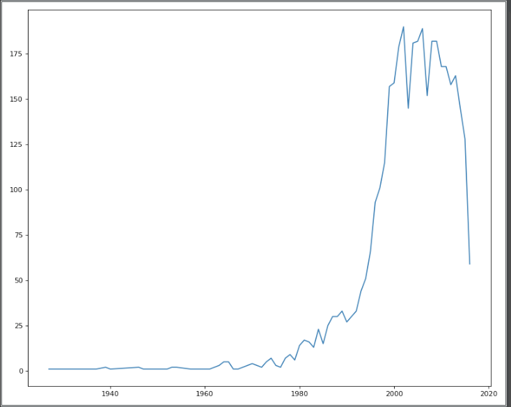
关于python pandas时间序列图,如何在ts.plot和之外设置xlim和xticks?的问题我们已经讲解完毕,感谢您的阅读,如果还想了解更多关于pandas小记:pandas时间序列分析和处理Timeseries、pandas时间序列之pd.to_datetime()的实现、pandas时间序列之如何将int转换成datetime格式、Pandas时间序列和分组聚合等相关内容,可以在本站寻找。
本文标签:


