关于macos–gobuildruntime:darwin/amd64必须使用make.bash进行引导的问题就给大家分享到这里,感谢你花时间阅读本站内容,更多关于bash–安装make命令没有mak
关于macos – go build runtime:darwin / amd64必须使用make.bash进行引导的问题就给大家分享到这里,感谢你花时间阅读本站内容,更多关于bash – 安装make命令没有make(mac os 10.5)、Build caffe using qmake (ubuntu&windows)、Building an AI-powered Battlesnake with reinforcement learning on Amazon SageMaker、Building real-time dashboard applications with Apache Flink, Elasticsearch, and Kibana等相关知识的信息别忘了在本站进行查找喔。
本文目录一览:- macos – go build runtime:darwin / amd64必须使用make.bash进行引导
- bash – 安装make命令没有make(mac os 10.5)
- Build caffe using qmake (ubuntu&windows)
- Building an AI-powered Battlesnake with reinforcement learning on Amazon SageMaker
- Building real-time dashboard applications with Apache Flink, Elasticsearch, and Kibana

macos – go build runtime:darwin / amd64必须使用make.bash进行引导
go build runtime: darwin/amd64 must be bootstrapped using make.bash
然后参考问题Cross compile Go on OSX?
我先尝试过:
brew install go --with-cc-all
但问题仍然存在,然后我尝试:
cd /usr/local/go/src
sudo GOOS=darwin GOARCH=amd64 CGO_ENABLED=0 ./make.bash --no-clean
但问题仍然存在.那么我该如何解决这个问题呢?
System Version: OS X 10.10.4 (14E46)
Kernel Version: Darwin 14.4.0
Go Version: go version go1.4.2 darwin/amd64
解决方法
从结帐源,在src中:
src $GOOS=darwin GOARCH=amd64 ./bootstrap.bash
#### copying to ../../go-darwin-amd64-bootstrap
...
----
Bootstrap toolchain for darwin/amd64 installed in XXX/go-darwin-amd64-bootstrap.
Building tbz.
-rw-r--r--  1 hvn  staff  48149988 Aug 21 10:48 XXX/go-darwin-amd64-bootstrap.tbz
然后我解压缩tbz并正常构建它:
$tar xzf XXX/go-darwin-amd64-bootstrap.tbz
cd到那个提取的目录.然后
$./all.bash
##### Building Go bootstrap tool.
cmd/dist
...

ALL TESTS PASSED

---
Installed Go for darwin/amd64...

$go-darwin-amd64-bootstrap/bin/go version
go version go1.5 darwin/amd64
希望有所帮助.
")
bash – 安装make命令没有make(mac os 10.5)
(我知道您可以通过安装 Xcode和Mac OS附带的开发人员工具来完成,但是我不希望人们去找到他们的mac os安装dvds以使用该脚本.)
它甚至不需要做,我只是寻找一个实用程序,您可以轻松地下载脚本(使用ftp或curl),并用于编译源代码.
If you need to build GNU Make and have no other make program to use,
you can use the shell script build.sh instead. To do this,first run
configureas described in INSTALL. Then,instead of typingmaketo
build the program,typesh build.sh. This should compile the program
in the current directory. Then you will have a Make program that you can
use for./make install,or whatever else.
是的,他们想到了这个问题!
")
Build caffe using qmake (ubuntu&windows)
1. Problem
I want to build caffe on windows. Windows official version is a little complex,since I need to change dependent libs frequently. For a cross-platform solution,Qt is an awesome choice.
2. Solution
Platform: Windows10(x64)+ VS2013 (msvc120)
2.1 Prepare
Caffe uses a lot of cpp libs: boost,gflags,glog,hdf5,LevelDB,Imdb,openblas,opencv,protobuf. I upload msvc120_x64 version here.
2.2 Code
Qt uses qmake to manage project. All you need just a *.pro file,as CMakeLists.txt for cmake.
Here is libcaffe.pro
TEMPLATE = lib
CONfig(debug,debug|release): TARGET = libcaffed
CONfig(release,debug|release): TARGET = libcaffe
INCLUDEPATH += include src include/caffe/proto
DEFInes += USE_OPENCV cpu_ONLY
CONfig += dll staticlib

# Input
HEADERS += \     include/caffe/blob.hpp\     include/caffe/caffe.hpp\     include/caffe/common.hpp\     include/caffe/data_reader.hpp\     include/caffe/data_transformer.hpp\     include/caffe/filler.hpp\     include/caffe/internal_thread.hpp\     include/caffe/layer.hpp\     include/caffe/layers/absval_layer.hpp\     include/caffe/layers/accuracy_layer.hpp\     include/caffe/layers/argmax_layer.hpp\     include/caffe/layers/base_conv_layer.hpp\     include/caffe/layers/base_data_layer.hpp\     include/caffe/layers/batch_norm_layer.hpp\     include/caffe/layers/batch_reindex_layer.hpp\     include/caffe/layers/bias_layer.hpp\     include/caffe/layers/bnll_layer.hpp\     include/caffe/layers/Box_annotator_ohem_layer.hpp\     include/caffe/layers/concat_layer.hpp\     include/caffe/layers/contrastive_loss_layer.hpp\     include/caffe/layers/conv_layer.hpp\     include/caffe/layers/crop_layer.hpp\     include/caffe/layers/cudnn_conv_layer.hpp\     include/caffe/layers/cudnn_lcn_layer.hpp\     include/caffe/layers/cudnn_lrn_layer.hpp\     include/caffe/layers/cudnn_pooling_layer.hpp\     include/caffe/layers/cudnn_relu_layer.hpp\     include/caffe/layers/cudnn_sigmoid_layer.hpp\     include/caffe/layers/cudnn_softmax_layer.hpp\     include/caffe/layers/cudnn_tanh_layer.hpp\     include/caffe/layers/data_layer.hpp\     include/caffe/layers/deconv_layer.hpp\     include/caffe/layers/dropout_layer.hpp\     include/caffe/layers/dummy_data_layer.hpp\     include/caffe/layers/eltwise_layer.hpp\     include/caffe/layers/elu_layer.hpp\     include/caffe/layers/embed_layer.hpp\     include/caffe/layers/euclidean_loss_layer.hpp\     include/caffe/layers/exp_layer.hpp\     include/caffe/layers/filter_layer.hpp\     include/caffe/layers/flatten_layer.hpp\     include/caffe/layers/hdf5_data_layer/.hpp\     include/caffe/layers/hdf5_output_layer.hpp\     include/caffe/layers/hinge_loss_layer.hpp\     include/caffe/layers/im2col_layer.hpp\     include/caffe/layers/image_data_layer.hpp\     include/caffe/layers/infogain_loss_layer.hpp\     include/caffe/layers/inner_product_layer.hpp\     include/caffe/layers/input_layer.hpp\     include/caffe/layers/log_layer.hpp\     include/caffe/layers/loss_layer.hpp\     include/caffe/layers/lrn_layer.hpp\     include/caffe/layers/lstm_layer.hpp\     include/caffe/layers/memory_data_layer.hpp\     include/caffe/layers/multinomial_logistic_loss_layer.hpp\     include/caffe/layers/mvn_layer.hpp\     include/caffe/layers/neuron_layer.hpp\     include/caffe/layers/parameter_layer.hpp\     include/caffe/layers/pooling_layer.hpp\     include/caffe/layers/power_layer.hpp\     include/caffe/layers/prelu_layer.hpp\     include/caffe/layers/psroi_pooling_layer.hpp\     include/caffe/layers/python_layer.hpp\     include/caffe/layers/recurrent_layer.hpp\     include/caffe/layers/reduction_layer.hpp\     include/caffe/layers/relu_layer.hpp\     include/caffe/layers/reshape_layer.hpp\     include/caffe/layers/rnn_layer.hpp\     include/caffe/layers/roi_pooling_layer.hpp\     include/caffe/layers/scale_layer.hpp\     include/caffe/layers/sigmoid_cross_entropy_loss_layer.hpp\     include/caffe/layers/sigmoid_layer.hpp\     include/caffe/layers/silence_layer.hpp\     include/caffe/layers/slice_layer.hpp\     include/caffe/layers/smooth_l1_loss_layer.hpp\     include/caffe/layers/smooth_l1_loss_ohem_layer.hpp\     include/caffe/layers/softmax_layer.hpp\     include/caffe/layers/softmax_loss_layer.hpp\     include/caffe/layers/softmax_loss_ohem_layer.hpp\     include/caffe/layers/split_layer.hpp\     include/caffe/layers/spp_layer.hpp\     include/caffe/layers/tanh_layer.hpp\     include/caffe/layers/threshold_layer.hpp\     include/caffe/layers/tile_layer.hpp\     include/caffe/layers/window_data_layer.hpp\     include/caffe/layer_factory.hpp\     include/caffe/net.hpp\     include/caffe/parallel.hpp\     include/caffe/proto/caffe.pb.h\     include/caffe/sgd_solvers.hpp\     include/caffe/solver.hpp\     include/caffe/solver_factory.hpp\     include/caffe/syncedmem.hpp\     include/caffe/util/benchmark.hpp\     include/caffe/util/blocking_queue.hpp\     include/caffe/util/cudnn.hpp\     include/caffe/util/db.hpp\     include/caffe/util/db_leveldb.hpp\     include/caffe/util/db_lmdb.hpp\     include/caffe/util/device_alternate.hpp\     include/caffe/util/format.hpp\     include/caffe/util/hdf5.hpp\     include/caffe/util/im2col.hpp\     include/caffe/util/insert_splits.hpp\     include/caffe/util/io.hpp\     include/caffe/util/math_functions.hpp\     include/caffe/util/mkl_alternate.hpp\     include/caffe/util/rng.hpp\     include/caffe/util/signal_handler.h\     include/caffe/util/upgrade_proto.hpp

SOURCES += \    src/caffe/blob.cpp \    src/caffe/common.cpp \    src/caffe/data_reader.cpp \    src/caffe/data_transformer.cpp \    src/caffe/internal_thread.cpp \    src/caffe/layer.cpp \    src/caffe/layers/absval_layer.cpp \    src/caffe/layers/accuracy_layer.cpp \    src/caffe/layers/argmax_layer.cpp \    src/caffe/layers/base_conv_layer.cpp \    src/caffe/layers/base_data_layer.cpp \    src/caffe/layers/batch_norm_layer.cpp \    src/caffe/layers/batch_reindex_layer.cpp \    src/caffe/layers/bias_layer.cpp \    src/caffe/layers/bnll_layer.cpp \    src/caffe/layers/Box_annotator_ohem_layer.cpp \    src/caffe/layers/concat_layer.cpp \    src/caffe/layers/contrastive_loss_layer.cpp \    src/caffe/layers/conv_layer.cpp \    src/caffe/layers/crop_layer.cpp \    src/caffe/layers/cudnn_conv_layer.cpp \    src/caffe/layers/cudnn_lcn_layer.cpp \    src/caffe/layers/cudnn_lrn_layer.cpp \    src/caffe/layers/cudnn_pooling_layer.cpp \    src/caffe/layers/cudnn_relu_layer.cpp \    src/caffe/layers/cudnn_sigmoid_layer.cpp \    src/caffe/layers/cudnn_softmax_layer.cpp \    src/caffe/layers/cudnn_tanh_layer.cpp \    src/caffe/layers/data_layer.cpp \    src/caffe/layers/deconv_layer.cpp \    src/caffe/layers/dropout_layer.cpp \    src/caffe/layers/dummy_data_layer.cpp \    src/caffe/layers/eltwise_layer.cpp \    src/caffe/layers/elu_layer.cpp \    src/caffe/layers/embed_layer.cpp \    src/caffe/layers/euclidean_loss_layer.cpp \    src/caffe/layers/exp_layer.cpp \    src/caffe/layers/filter_layer.cpp \    src/caffe/layers/flatten_layer.cpp \    src/caffe/layers/hdf5_data_layer.cpp \    src/caffe/layers/hdf5_output_layer.cpp \    src/caffe/layers/hinge_loss_layer.cpp \    src/caffe/layers/im2col_layer.cpp \    src/caffe/layers/image_data_layer.cpp \    src/caffe/layers/infogain_loss_layer.cpp \    src/caffe/layers/inner_product_layer.cpp \    src/caffe/layers/input_layer.cpp \    src/caffe/layers/log_layer.cpp \    src/caffe/layers/loss_layer.cpp \    src/caffe/layers/lrn_layer.cpp \    src/caffe/layers/lstm_layer.cpp \    src/caffe/layers/lstm_unit_layer.cpp \    src/caffe/layers/memory_data_layer.cpp \    src/caffe/layers/multinomial_logistic_loss_layer.cpp \    src/caffe/layers/mvn_layer.cpp \    src/caffe/layers/neuron_layer.cpp \    src/caffe/layers/parameter_layer.cpp \    src/caffe/layers/pooling_layer.cpp \    src/caffe/layers/power_layer.cpp \    src/caffe/layers/prelu_layer.cpp \    src/caffe/layers/psroi_pooling_layer.cpp \    src/caffe/layers/recurrent_layer.cpp \    src/caffe/layers/reduction_layer.cpp \    src/caffe/layers/relu_layer.cpp \    src/caffe/layers/reshape_layer.cpp \    src/caffe/layers/rnn_layer.cpp \    src/caffe/layers/roi_pooling_layer.cpp \    src/caffe/layers/scale_layer.cpp \    src/caffe/layers/sigmoid_cross_entropy_loss_layer.cpp \    src/caffe/layers/sigmoid_layer.cpp \    src/caffe/layers/silence_layer.cpp \    src/caffe/layers/slice_layer.cpp \    src/caffe/layers/smooth_l1_loss_layer.cpp \    src/caffe/layers/smooth_L1_loss_ohem_layer.cpp \    src/caffe/layers/softmax_layer.cpp \    src/caffe/layers/softmax_loss_layer.cpp \    src/caffe/layers/softmax_loss_ohem_layer.cpp \    src/caffe/layers/split_layer.cpp \    src/caffe/layers/spp_layer.cpp \    src/caffe/layers/tanh_layer.cpp \    src/caffe/layers/threshold_layer.cpp \    src/caffe/layers/tile_layer.cpp \    src/caffe/layers/window_data_layer.cpp \    src/caffe/layer_factory.cpp \    src/caffe/net.cpp \    src/caffe/parallel.cpp \    src/caffe/solver.cpp \    src/caffe/solvers/adadelta_solver.cpp \    src/caffe/solvers/adagrad_solver.cpp \    src/caffe/solvers/adam_solver.cpp \    src/caffe/solvers/nesterov_solver.cpp \    src/caffe/solvers/rmsprop_solver.cpp \    src/caffe/solvers/sgd_solver.cpp \    src/caffe/syncedmem.cpp \    src/caffe/util/benchmark.cpp \    src/caffe/util/blocking_queue.cpp \    src/caffe/util/cudnn.cpp \    src/caffe/util/db.cpp \    src/caffe/util/db_leveldb.cpp \    src/caffe/util/db_lmdb.cpp \    src/caffe/util/hdf5.cpp \    src/caffe/util/im2col.cpp \    src/caffe/util/insert_splits.cpp \    src/caffe/util/io.cpp \    src/caffe/util/math_functions.cpp \    src/caffe/util/signal_handler.cpp \    src/caffe/util/upgrade_proto.cpp \    src/caffe/proto/caffe.pb.cc

win32{

# opencv
PATH_OPENCV_INCLUDE   = "H:\3rdparty\OpenCV\opencv310\build\include"
PATH_OPENCV_LIBRARIES = "H:\3rdparty\OpenCV\opencv310\build\x64\vc12\lib"
VERSION_OPENCV        = 310
INCLUDEPATH += $${PATH_OPENCV_INCLUDE} CONfig(debug,debug|release){ LIBS += -L$${PATH_OPENCV_LIBRARIES} -lopencv_core$${VERSION_OPENCV}d LIBS += -L$${PATH_OPENCV_LIBRARIES} -lopencv_highgui$${VERSION_OPENCV}d LIBS += -L$${PATH_OPENCV_LIBRARIES} -lopencv_imgcodecs$${VERSION_OPENCV}d LIBS += -L$${PATH_OPENCV_LIBRARIES} -lopencv_imgproc$${VERSION_OPENCV}d } CONfig(release,debug|release){ LIBS += -L$${PATH_OPENCV_LIBRARIES} -lopencv_core$${VERSION_OPENCV} LIBS += -L$${PATH_OPENCV_LIBRARIES} -lopencv_highgui$${VERSION_OPENCV} LIBS += -L$${PATH_OPENCV_LIBRARIES} -lopencv_imgcodecs$${VERSION_OPENCV} LIBS += -L$${PATH_OPENCV_LIBRARIES} -lopencv_imgproc$${VERSION_OPENCV} } #glog INCLUDEPATH += H:\3rdparty\glog\include LIBS += -LH:\3rdparty\glog\lib\x64\v120\Debug\dynamic -llibglog #boost INCLUDEPATH += H:\3rdparty\boost\boost_1_59_0 CONfig(debug,debug|release): BOOST_VERSION = "-vc120-mt-gd-1_59" CONfig(release,debug|release): BOOST_VERSION = "-vc120-mt-1_59" LIBS += -LH:\3rdparty\boost\boost_1_59_0\lib64-msvc-12.0 \  -llibboost_system$${BOOST_VERSION} \     -llibboost_date_time$${BOOST_VERSION} \  -llibboost_filesystem$${BOOST_VERSION} \     -llibboost_thread$${BOOST_VERSION} \  -llibboost_regex$${BOOST_VERSION}

#gflags
INCLUDEPATH += H:\3rdparty\gflags\include
CONfig(debug,debug|release): LIBS += -LH:\3rdparty\gflags\x64\v120\dynamic\Lib -lgflagsd
CONfig(release,debug|release): LIBS += -LH:\3rdparty\gflags\x64\v120\dynamic\Lib -lgflags

#protobuf
INCLUDEPATH += H:\3rdparty\protobuf\include
CONfig(debug,debug|release): LIBS += -LH:\3rdparty\protobuf\lib\x64\v120\Debug -llibprotobuf
CONfig(release,debug|release): LIBS += -LH:\3rdparty\protobuf\lib\x64\v120\Release -llibprotobuf

# hdf5
INCLUDEPATH += H:\3rdparty\hdf5\include
LIBS += -LH:\3rdparty\hdf5\lib\x64 -lhdf5 -lhdf5_hl -lhdf5_tools -lhdf5_cpp

# levelDb
INCLUDEPATH += H:\3rdparty\LevelDB\include
CONfig(debug,debug|release): LIBS += -LH:\3rdparty\LevelDB\lib\x64\v120\Debug -lLevelDb
CONfig(release,debug|release): LIBS += -LH:\3rdparty\LevelDB\lib\x64\v120\Release -lLevelDb

# lmdb
INCLUDEPATH += H:\3rdparty\lmdb\include
CONfig(debug,debug|release): LIBS += -LH:\3rdparty\lmdb\lib\x64 -llmdbD
CONfig(release,debug|release): LIBS += -LH:\3rdparty\lmdb\lib\x64 -llmdb

#openblas
INCLUDEPATH += H:\3rdparty\openblas\include
LIBS += -LH:\3rdparty\openblas\lib\x64 -llibopenblas
}
You neeed to change library path to your own.
Done.
You can find caffe project on my github

Building an AI-powered Battlesnake with reinforcement learning on Amazon SageMaker
https://amazonaws-china.com/blogs/machine-learning/building-an-ai-powered-battlesnake-with-reinforcement-learning-on-amazon-sagemaker/
Battlesnake is an AI competition based on the traditional snake game in which multiple AI-powered snakes compete to be the last snake surviving. Battlesnake attracts a community of developers at all levels. Hundreds of snakes compete and rise up in the ranks in the online Battlesnake global arena. Battlesnake also hosts several offline events that are attended by more than a thousand developers and non-developers alike and are streamed on Twitch. Teams of developers build snakes for the competition and learn new tech skills, learn to collaborate, and have fun. Teams can build snakes by using a variety of strategies ranging from state-of-the-art deep reinforcement learning (RL) algorithms to unique heuristics-based strategies.
This post shows how to use Amazon SageMaker to build an RL-based snake.
In the traditional snake game, you control your snakes to move up, down, left, or right. If your snake hits a wall, another snake, or your snake’s own body, your snake dies. When your snake eats food, it grows longer. In Battlesnake, there are several differences compared to the traditional snake game. Firstly, programs control the snakes. When two snakes have a head-on collision, the smaller snake dies. Also, there is a starvation mechanism. Snakes that haven’t had food for 100 moves die. Therefore, maximizing survivability, aggressively attacking other snakes, or trying to avoid other snakes are all viable strategies that players have adopted. The snakes are implemented as a programmed web server that the Battlesnake engine queries for the next move given the current state of the game. For more information, see Getting Started on the Battlesnake website.
This post shows how to use the SageMaker Battlesnake Starter Pack to reduce the time and effort required to build your snakes. The SageMaker Battlesnake Starter Pack provides you with an AI-powered snake trained with RL. The Starter Pack also provides an environment for you to train your own RL policy and the tools to build custom heuristics-based rules on top of the RL algorithms. Furthermore, the web infrastructure to deploy and host your AI bot are generated automatically. The SageMaker Battlesnake Starter Pack allows you to focus on developing your AI instead of worrying about the infrastructure surrounding it.
The Amazon SageMaker Battlesnake Starter Pack uses quick-create links in AWS CloudFormation, which provide one-click deployment from the GitHub repo to your AWS Management Console. The creation of the stack deploys the following three layers and a development environment:
- The first layer is an Amazon API Gateway, which exposes the snake HTTP API to the Battlesnake engine
- The second layer is an AWS Lambda function that transcribes the Battlesnake API into the RL agent’s internal representation
- The third layer is an Amazon SageMaker endpoint that hosts the snake
- The development environment is made of Jupyter notebooks that run inside an Amazon SageMaker notebook instance
The following diagram illustrates the runtime AI infrastructure.
The SageMaker Battlesnake Starter Pack does the following:
- Allows you to deploy the framework, which includes the development environment and an AI-powered snake
- Provides you with tools to modify and evaluate new heuristic-based rules to alter your snake’s behavior
- Includes training scripts to retrain and optimize a custom RL agent
By the end of this post, you should understand the basics of RL and how to model Battlesnake in an RL framework, and have a snake that can compete against other snakes in the online global arena.
Reinforcement learning with Battlesnake
This section reviews the basics of reinforcement learning and how the SageMaker Battlesnake Starter Pack models the Battlesnake environment in an RL framework.
Introduction to reinforcement learning
Reinforcement learning develops strategies for sequential decision-making problems. Given a pre-specified reward signal, the RL agent interacts with the environment. Its goal is to make actions based on the state it receives, and to maximize the expected cumulative reward. The strategy to take actions is called a policy (π(a|s)). Assume you have a starting point t=0 and an ending point t=T (your snake dies). Each game creates an episode that contains a list of states (st), actions (at), rewards (rt), and next states (st+1). Therefore, you can express the cumulative reward as the following equation:

In this equation, γ is the discount factor for future rewards.
For more information on RL concepts and mathematical formulation, see Automating financial decision making with deep reinforcement learning.
Understanding the Battlesnake environment
Building a Battlesnake agent requires an extension of the described RL framework to accommodate for multiple agents. The following diagram illustrates a multi-agent RL problem to train a Battlesnake agent.

With the SageMaker Battlesnake Starter Pack, you can customize your environment through the open-source OpenAI Gym interface. A custom file called snake_gym.py is located in the LocalEnv/battlesnake_gym/battlesnake_gym/folder and specifies all the entities discussed previously. The following code defines the state space (which is defined by the map_size, number and location of snakes, and location of food, and is denoted as observation_space) and the action space (up, down, left, right):
# Custom environment file in Open AI Gym

class BattlesnakeGym(gym.Env):
    def __init__(self, observation_type="flat-51s", map_size=(15, 15),
                 number_of_snakes=4,
                 snake_spawn_locations=[], food_spawn_locations=[],
                 verbose=False, initial_game_state=None, rewards=SimpleRewards()):

        # Action space
        self.action_space = MultiAgentActionSpace(
            [spaces.Discrete(4) for _ in range(number_of_snakes)])

        # Observation space
        self.observation_type = observation_type
        if "flat" in self.observation_type:
            self.observation_space = spaces.Box(low=0, high=2,
                                                shape=(self.map_size[0],
                                                       self.map_size[1],
                                                       self.number_of_snakes+1),
                                                dtype=np.uint8)
        elif "bordered" in self.observation_type:
            self.observation_space = spaces.Box(low=0, high=2,
                                                shape=(self.map_size[0]+2,
                                                       self.map_size[1]+2,
                                                       self.number_of_snakes+1),
                                                dtype=np.uint8)

        (...)
The default state representation of the Battlesnake gym is to use a multi-channel image, in which the first channel represents the food positions, the second channel indicates the position of the snake your agent is controlling, and the third channel represents the positions of the other snakes. The representation of the environment is defined in LocalEnv/battlesnake_gym/battlesnake_gym/snake.py. See the following image.

The step() method takes the actions performed by each snake and runs the state transition to get the resulting new state and rewards. You can define your state transitions with the following code:
def step(self, actions, episodes=None):
    # setup reward dict
    reward = {}
    snake_info = {}

    # Reduce health and move
    for i, snake in enumerate(self.snakes.get_snakes()):
        reward[i] = 0
        if not snake.is_alive():
            continue

        # Reduce health by one
        snake.health -= 1
        if snake.health == 0:
            snake.kill_snake()
            reward[i] += self.rewards.get_reward("starved", i, episodes)
            snake_info[i] = "starved"
            continue

        action = actions[i]
        is_forbidden = snake.move(action)
        if is_forbidden:
            snake.kill_snake()
            reward[i] += self.rewards.get_reward("forbidden_move", i, episodes)
            snake_info[i] = "forbidden move"

    # check for food and collision
    (...)

    return self._get_observation(), reward, snake_alive_dict, {''current_turn'': self.turn_count,
                                                                ''snake_health'': snakes_health,
                                                                ''snake_info'': snake_info}
You can customize your reward function in LocalEnv/battlesnake_gym/battlesnake_gym/rewards.py. By default, the gym supports the following reward definitions:
- Surviving another turn (
"another_turn") - Eating food (
"ate_food") - Winning the game (
"won") - Losing the game (
"died") - Eating another snake (
"ate_another_snake") - Hitting a wall (
"hit_wall") - Hitting another snake (
"hit_other_snake") - Hitting yourself (
"hit_self") - Being eaten by another snake (
"was_eaten") - Getting hit by another snake (
"other_snake_hit_body") - Performing a forbidden move, such as moving south when facing north (
"forbidden_move") - Dying by starving (
"starved")
Reinforcement learning algorithm
There are many algorithms with which to learn an RL policy. The SageMaker Battlesnake Starter Pack provides a classic method called deep Q-learning (DQN). The Q stands for quality and represents how good a given action a is in gaining future rewards given the current state s. Mathematically, the Q-value is defined as the following equation:
![]()
In this equation, s’ denotes the next state. Essentially, you consider all possible actions and all possible next states in the preceding equation, and then you take the maximum value given by taking a certain action.
Q(s’,a) again depends on Q(s”,a) . Therefore, the Q-value depends on Q-values of all future states. See the following equation:
![]()
We learn the Q function using the following equation:
![]()
In this equation, α is the learning rate. The updating process is called Q-learning. It enables you to update the Q-value based on the current Q-value at timestep t and the Q-value at t+1, and α controls to what extent newly acquired information overrides the old information. Theoretical analysis has proven that under mild conditions of α, the update converges to the optimal policy π*, assuming infinite random action selection.
In practice, the environment can have a considerable number of states, and it’s not feasible to record all Q-values in the table. This is also true for Battlesnake because the input is an image of the current state. The amount of memory and time required to save and update the Q-table is unrealistic because every input image can be different. To mitigate this issue, you can approximate the Q-values with a neural network, and this leads to the deep Q-learning. Specifically, the game state is provided as the input, and the Q-values of all possible actions is served as the output. This post provides an attention- and concatenation-based Q-network, which you can use as-is or as the starting point for your custom snake. You can find the network in qnetworks.py under LocalEnv/battlesnake_src/networks/.
The SageMaker Battlesnake Starter Pack includes a model trained on the described RL framework. This post includes the following steps:
- Deploying this trained model and a development environment with which you can improve it
- Evaluating new heuristic-based rules to customize your snake’s behavior
- Customizing and tuning your RL algorithm
Step 1: Deploying the Amazon SageMaker Battlesnake Starter Pack
This section contains the following steps:
- Launch the Amazon SageMaker Battlesnake Starter Pack to deploy a starter snake and the development environment to customize the snake.
- Link the API Gateway to the Battlesnake engine. The snake is then available to compete in the Battlesnake arena.
Deploying the Battlesnake Starter Pack
To deploy the Starter Pack, complete the following steps:
- Navigate to Deploy environment in the GitHub repo.
- Choose deploy in your desired Region.
The Battlesnake engine runs on us-west-2; you may want to deploy in the same Region to have the lowest latency.
After you choose deploy, you should be in the CloudFormation stack creation process.
- In Parameters, you can define the default Amazon EC2 instance types to use.
Instance types m5.xlarge and m4.xlarge are a part of the free tier of Amazon SageMaker. However, they are not available to new AWS accounts by default. If you are new to AWS, you can instead use a t2.medium instance, which is both cost-effective and sufficiently powerful for the Battlesnake use case.
- In Parameters, you can also define your snake’s color, head style, and tail style.
You should see the following image of snakes in different colors and styles.

The following screenshot shows the different snake styles you can choose from.

For more information, see Customizing Your Snake on the Battlesnake website.
- In the Capabilities and transforms section, select all the permissions.
- Choose Create stack.
You are now on the BattlesnakeEnvironment creation page. After about 10 minutes, you see the status CREATE_COMPLETE.
If you ever need to navigate to the stack again, navigate to the AWS CloudFormation console and choose BattlesnakeEnvironment.
- On the Outputs tab, choose the link next to CheckSnakeStatus.

You should be redirected to a webpage indicating the status of the snake creation. The following lines show an example of the webpage when the snake is being created.
snake status : not ready
Sagemaker endpoint status : Creating
You can visit the Amazon SageMaker service page in the AWS Management Console to see detailed information.
After approximately 15 minutes, you should see snake status : ready, which indicates that the Amazon SageMaker endpoint creation is complete. You now have a deployed web server that can respond to the Battlesnake engine.
To create a snake and link it to the Battlesnake engine, complete the following steps:
- Create a snake on the Battlesnake website.
- For Name, enter your desired name.
- For URL, enter the URL for your SnakeAPI.
The URL is available on the Outputs tab of your CloudFormation stack.
- Optionally, enter a description and tags.
- Optionally, select if others can add your snake to a game.
- Choose Save.

You can now test your snake against existing snakes. The following video shows a game of Battlesnake.
The snake My SageMaker Snake is slow but steady, and ultimately wins. For more information, see the details of this game on the Battlesnake website.
The following screencast shows the full procedures of this step. The video has been edited to skip the wait time.
Navigating the development environment
Now that you have a working snake, you can start exploring the development environment. On the Outputs tab of the CloudFormation stack, you can see the following keys:
- SourceEditionInNotebook – A link to the source directory of the development environment in a Jupyter notebook.
- HeuristicsDevEnvironment – A link to the heuristics development notebook. Details are in Step 2 of this post.
- ModelTrainingEnvironment – A link to the RL training notebook. Details are in Step 3 of this post.
The Starter Pack environment
The Starter Pack creates a local development directory. You can access it by opening the SourceEditionInNotebook and navigating to battlesnake/LocalEnv.
In LocalEnv, you can modify the following files to customize the SageMaker Starter Pack training, heuristics development, and evaluations:
- battlesnake_gym/battlesnake_gym/ – Files in this directory define the Battlesnake RL environment based on the OpenAI gym. This directory is copied into the Amazon SageMaker training job. It contains the following files:
food.pyhandles the food spawning mechanism and food representation.rewards.pydefines the reward function.snake.pydefines the snake movement mechanism, representation, and death conditions.snake_gym.pydefines the interactions between the snakes, food, and environment. The RL agents also interact with this file.
- battlesnake_inference/ – Files in this directory define the Amazon SageMaker endpoint used for inference of the model. It includes the following files:
battlesnake_heuristics.pydefines custom user-defined rules that can override the decision of the RL agent.predict.pyis the entry point to the Amazon SageMaker endpoint. It loads the network artifacts, obtains the decisions from the network, and activates the heuristics module.
- battlesnake_src/ – Files in this directory define the RL training jobs. This directory is copied into the Amazon SageMaker training job. It contains the following files:
train.pyis the entry point to the training job. It defines the hyperparameters of the agent and the environment. It also initiates the training loop.dqn_run.pydefines the deep Q-learning training loop.networks/agent.pydefines the RL agent. The agent performs the interaction between the Q network and the environment (to get an action and to learn).networks/qnetworks.pydefines the neural network (Q network) that the RL agent uses.
Step 2: Customizing your snake’s behavior
This section demonstrates how to write the heuristics that serve as ground rules for your snake. These ground rules override certain detrimental decisions that the deep learning model makes. For example, the following screenshot shows two snakes. If your snake (the shorter one) is in a situation where one decision leads to certain death (going down and hitting the longer snake), heuristics-based rules make sure that your snake goes up instead.

Other examples include rules that determine if a given movement decision results in a collision with a wall or if your snake can eat a shorter snake.
The heuristics-based rules are invoked within the Amazon SageMaker endpoint. The endpoint queries the deep learning model for an action. The action from the deep learning model and the state of the environment are fed into the heuristics code for any overriding actions.

Developing your heuristics
To develop your heuristics, open the heuristic development notebook (defined in HeuristicsDevEnvironment). This notebook simulates your model (with your heuristics), provides you with step-by-step visualization of your snakes, and deploys your new heuristics.
You can find a template for the heuristics code in LocalEnv/battlesnake_inference/battlesnake_heuristics.py. This consists of a class with a main run function. See the following code:
import numpy as np
import random

class MyBattlesnakeHeuristics:
    ''''''
    The BattlesnakeHeuristics class allows you to define handcrafted rules of the snake.
    ''''''
    FOOD_INDEX = 0
    def __init__(self):
        pass

    def go_to_food_if_close(self, state, json):
        # Example heuristic to move towards food if it''s close to you.

        # Get the position of the snake head
        your_snake_body = json["you"]["body"]
        i, j = your_snake_body[0]["y"], your_snake_body[0]["x"]

        # Set food_direction towards food
        food = state[:, :, self.FOOD_INDEX]

        # Note that there is a -1 border around state so i = i + 1, j = j + 1
        if -1 in state:
            i, j = i+1, j+1

        food_direction = None
        if food[i-1, j] == 1:
            food_direction = 0 # up
        if food[i+1, j] == 1:
            food_direction = 1 # down
        if food[i, j-1] == 1:
            food_direction = 2 # left
        if food[i, j+1] == 1:
            food_direction = 3 # right
        return food_direction

    def run(self, state, snake_id, turn_count, health, json, action):
        ''''''
        The main function of the heuristics.

        Parameters:
        -----------
        `state`: np.array of size (map_size[0]+2, map_size[1]+2, 1+number_of_snakes)
        Provides the current observation of the gym.
        Your target snake is state[:, :, snake_id+1]

        `snake_id`: int
        Indicates the id where id \in [0...number_of_snakes]

        `turn_count`: int
        Indicates the number of elapsed turns

        `health`: dict
        Indicates the health of all snakes in the form of {int: snake_id: int:health}

        `json`: dict
        Provides the same information as above, in the same format as the battlesnake engine.

        `action`: np.array of size 4
        The qvalues of the actions calculated. The 4 values correspond to [up, down, left, right]
        ''''''
        log_string = ""
        # The default `best_action` to take is the one that provides has the largest Q value.
        # If you think of something else, you can edit how `best_action` is calculated
        best_action = int(np.argmax(action))

        # Example heuristics to eat food that you are close to.
        if health[snake_id] < 30:
            food_direction = self.go_to_food_if_close(state, json)
            if food_direction:
                best_action = food_direction
                log_string = "Went to food if close."

        # TO DO, add your own heuristics

        assert best_action in [0, 1, 2, 3], "{} is not a valid action.".format(best_action)
        return best_action, log_string
Before you start writing your own heuristics, however, please read through the rest of Step 2.
The run function takes in the representation of the environment as the following arguments:
- state – An image format that can represent the environment
- json – A dictionary format that can also represent the environment
- snake_id – An integer indicating the ID of the snake
- turn_count – An integer indicating the current turn count
- health – A dictionary that represents the health of each snake
- action – A numpy array (of size 4) that provides the Q-values that represent the four possible actions (up, down, left, right), which is the output of the neural network.
In the preceding code, you can see a simple example heuristic, go_to_food_if_close. When your snake’s health is below 30 and there is food beside your snake, your snake moves towards the food. The purpose of this rule is to reduce the chances of your snake starving to death.
To write your own heuristics, you have to understand the advantages and disadvantages of using each representation of the environment. For example, the image representation is good when you are exploring possible moves or distances between different coordinates (such as determining if your snake is adjacent to a wall). However, the order of the snake body is lost in the image representation. The dictionary representation provides easy access to the head and tail of each snake. The example heuristics showcase the advantages of each representation method.
The snake head was obtained from the json argument (i, j = your_snake_body[0]["y"], your_snake_body[0]["x"]). Conversely, if you wanted to get the coordinates of the head in the image representation, you need an o(m*n) algorithm to iterate through the image to search for the head.
The direction of movements towards nearby food is obtained from the image representation (if food[i-1, j] == 1: ...). To use the json argument to search for the food, you have to use an o(n) algorithm to iterate through the list of foods for each possible direction.
Therefore, balancing between using the json list definitions and the state image allows you to write heuristic-based rules that override the decisions of the model.
Testing your heuristics
To evaluate your heuristics, you can use the heuristic development notebook. This notebook simulates the model with your heuristics and provides a step-by-step playback of all events. Firstly, define the initial conditions of the environment in the Define the openAI gym section of the notebook. To define the initial condition, set USE_INITIAL_STATE to be True and specify the coordinates of the food and snakes based on the Battlesnake API. Note that there is an easy way to define the initial_state here. See the following code:
USE_INITIAL_STATE = False

# Sample initial state for the situation simulator
initial_state = {
    "turn": 4,
    "board": {
                "height": 11,
                "width": 11,
                "food": [{"x": 1, "y": 3}],
                "snakes": [{
                                "health": 90,
                                "body": [{"x": 8, "y": 5}],
                           },
                           {
                                "health": 90,
                                "body": [{"x": 1, "y": 6}],
                           },
                           {
                                "health": 90,
                                "body": [{"x": 3, "y": 3}],
                            },
                            {
                                "health": 90,
                                "body": [{"x": 6, "y": 4}],
                            },
                            ]
            }
}

if USE_INITIAL_STATE == False:
    initial_state = None

map_size = (11, 11)
number_of_snakes = 4
env = BattlesnakeGym(map_size=map_size, number_of_snakes=number_of_snakes, observation_type="bordered-51s",
                     initial_game_state=initial_state)
Proceeding through the notebook loads the trained neural network and simulates the actions of each snake. You can see the step-by-step visualizer after you run the cells in the Playback the simulation section. The following screencast of the visualizer shows each step iterated step-by-step, then plays automatically.
During the visualization process, if you find that your snake cannot handle certain situations, you can run the following cell containing get_env_json(). This prints out a dictionary that represents the current state of the environment. You can directly copy the dictionary into the initial_state in the Define the openAI gym section and write specific heuristics to address the issues with the certain situation.
Deploying your heuristics
After you have finished with your heuristics, you can create an Amazon SageMaker endpoint with the new heuristics. Define the Amazon SageMaker session and only run the cell titled “Run if you retrained the model” if you have any trained model artifacts that you did not upload (see Step 3 in this post for more details). Continue to proceed through the notebook to update your Amazon SageMaker endpoint.
The deployment of your new Amazon SageMaker endpoint takes up to 10–15 minutes and you do not need to update your snake on the Battlesnake engine.
Step 3: Customizing the reinforcement learning training environment
This section shows how to train your deep RL for Battlesnake, perform hyperparameter optimization (HPO) to find the best model, and deploy the updated model into an Amazon SageMaker endpoint.
Training your model
In this step, you use the SagemakerModelTraining notebook (defined in ModelTrainingEnvironment). You can define the following two parameters of the notebook:
- The
run_hpoflag determines whether you should run a single training job or run HPO. - The
map_sizeparameter determines the size of the map for the environment to train on. The current neural network is limited to a single map size.
See the following code:
run_hpo = False
map_size = (15, 15)
You can define the hyperparameters to train in the cell Define the hyperparameters of your job. For more information on the details of each parameter, see the GitHub repo. See the following code:
map_size_string = "[{}, {}]".format(map_size[0], map_size[1])
static_hyperparameters = {
    ''qnetwork_type'': "attention",
    ''seed'': 111,
    ''number_of_snakes'': 4,
    ''episodes'': 10000,
    ''print_score_steps'': 10,
    ''activation_type'': "softrelu",
    ''state_type'': ''one_versus_all'',
    ''sequence_length'': 2,
    ''repeat_size'': 3,
    ''kernel_size'': 3,
    ''starting_channels'': 6,
    ''map_size'': map_size_string,
    ''snake_representation'': ''bordered-51s'',
    ''save_model_every'': 700,
    ''eps_start'': 0.99,
    ''models_to_save'': ''local''
}
You can create an MXNet estimator in the Train your model here cell to launch a training job. This process could take several hours, depending on your instance type. See the following code:
estimator = MXNet(entry_point="train.py",
                  source_dir=''battlesnake_src'',
                  dependencies=["battlesnake_gym/"],
                  role=role,
                  train_instance_type=train_instance_type,
                  train_instance_count=1,
                  output_path=s3_output_path,
                  framework_version="1.6.0",
                  py_version=''py3'',
                  base_job_name=job_name_prefix,
                  metric_definitions=metric_definitions,
                  hyperparameters=static_hyperparameters
                 )

estimator.fit()
You should see a training job with the prefix job_name_prefix launched on the Training Jobs session tab in the Amazon SageMaker console. After you choose the training job, you can see detailed information about the training run, for example, Amazon CloudWatch logs, real-time visualization of the metrics defined by metric_definitions, and the Amazon S3 location link for model output and artifacts.
Tuning your model
If you run an HPO job, you have to define hyperparameter ranges to iterate through. You can also perform hyperparameter optimization on the static_hyperparameters that were previously defined. See the following code:
hyperparameter_ranges = {
    ''buffer_size'': IntegerParameter(1000, 6000),
    ''update_every'': IntegerParameter(10, 20),
    ''batch_size'': IntegerParameter(16, 256),

    ''lr_start'': ContinuousParameter(1e-5, 1e-3),
    ''lr_factor'': ContinuousParameter(0.5, 1.0),
    ''lr_step'': IntegerParameter(5000, 30000),

    ''tau'': ContinuousParameter(1e-4, 1e-3),
    ''gamma'': ContinuousParameter(0.85, 0.99),

    ''depth'': IntegerParameter(10, 256),
    ''depthS'': IntegerParameter(10, 256),
}
Whether you chose to run HPO or a single training job, the model artifacts are saved on Amazon S3. This notebook automatically downloads the trained model artifacts from Amazon S3, packages it, and processes it for updating the Amazon SageMaker endpoint automatically. You do not have to update your snake on the Battlesnake engine.
Conclusion
The mission of Battlesnake is for developers of all levels to have fun with friends, learn new skills, and build a community. The SageMaker Battlesnake Starter Pack builds on this mission to encompass developers at all levels. Whether you want to build a snake based on decision trees or RL, you can use the SageMaker Battlesnake Starter Pack.
This post showed you how to deploy a snake in the Battlesnake arena to compete against other snakes and the development environment to modify and upgrade the models with your custom configuration. Historically, snakes built with heuristics-based decisions tree outperformed machine learning-based snakes in the offline Battlesnake competitions. Lately, there’s a trend that RL-based snakes are rising up in the ranks in the online global arena. Try out the SageMaker Battlesnake Starter Pack and see if this year a hybrid RL and heuristics snake can take the win!
About the Authors
 Jonathan Chung is an Applied scientist in AWS. He works on applying deep learning to various applications including games and document analysis. He enjoys cooking and visiting historical cities around the world.
 Xavier Raffin is a Solutions Architect at AWS where he helps customers to transform their businesses and build industry leading cloud solutions. Xavier curiosity, pushed him to apply technology onto many domains: Public Transportation, Web Mapping, IoT, Aeronautics and Space. He contributed to several OpenSource and Opendata projects: OpenStreetMap, Navitia, Transport APIs.
 Anna Luo is an Applied Scientist in AWS. She works on utilizing reinforcement learning techniques for different domains including supply chain and recommender system. Her current personal goal is to master snowboarding.
 Bharathan Balaji is a Research Scientist in AWS and his research interests lie in reinforcement learning systems and applications. He contributed to the launch of Amazon SageMaker RL and AWS DeepRacer. He likes to play badminton, cricket and board games during his spare time.
 Vishaal Kapoor is a Senior Software Development Manager with AWS AI. He loves all things AI and works on building deep learning solutions using SageMaker. In his spare time, he mountain bikes, snowboards, and spends time with his family.

Building real-time dashboard applications with Apache Flink, Elasticsearch, and Kibana
https://www.elastic.co/cn/blog/building-real-time-dashboard-applications-with-apache-flink-elasticsearch-and-kibana
Fabian Hueske
Share
Gaining actionable insights from continuously produced data in real-time is a common requirement for many businesses today. A wide-spread use case for real-time data processing is dashboarding. A typical architecture to support such a use case is based on a data stream processor, a data store with low latency read/write access, and a visualization framework.
In this blog post, we demonstrate how to build a real-time dashboard solution for stream data analytics using Apache Flink, Elasticsearch, and Kibana. The following figure depicts our system architecture.
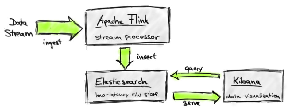
In our architecture, Apache Flink executes stream analysis jobs that ingest a data stream, apply transformations to analyze, transform, and model the data in motion, and write their results to an Elasticsearch index. Kibana connects to the index and queries it for data to visualize. All components of our architecture are open source systems under the Apache License 2.0. We show how to implement a Flink DataStream program that analyzes a stream of taxi ride events and writes its results to Elasticsearch and give instructions on how to connect and configure Kibana to visualize the analyzed data in real-time.
Why use Apache Flink for stream processing?
Before we dive into the details of implementing our demo application, we discuss some of the features that make Apache Flink an outstanding stream processor. Apache Flink 0.10, which was recently released, comes with a competitive set of stream processing features, some of which are unique in the open source domain. The most important ones are:
- Support for event time and out of order streams: In reality, streams of events rarely arrive in the order that they are produced, especially streams from distributed systems and devices. Until now, it was up to the application programmer to correct this “time drift”, or simply ignore it and accept inaccurate results, as streaming systems (at least in the open source world) had no support for event time (i.e., processing events by the time they happened in the real world). Flink 0.10 is the first open source engine that supports out of order streams and which is able to consistently process events according to their timestamps.
- Expressive and easy-to-use APIs in Scala and Java: Flink''s DataStream API ports many operators which are well known from batch processing APIs such as map, reduce, and join to the streaming world. In addition, it provides stream-specific operations such as window, split, and connect. First-class support for user-defined functions eases the implementation of custom application behavior. The DataStream API is available in Scala and Java.
- Support for sessions and unaligned windows: Most streaming systems have some concept of windowing, i.e., a grouping of events based on some function of time. Unfortunately, in many systems these windows are hard-coded and connected with the system’s internal checkpointing mechanism. Flink is the first open source streaming engine that completely decouples windowing from fault tolerance, allowing for richer forms of windows, such as sessions.
- Consistency, fault tolerance, and high availability: Flink guarantees consistent state updates in the presence of failures (often called “exactly-once processing”), and consistent data movement between selected sources and sinks (e.g., consistent data movement between Kafka and HDFS). Flink also supports worker and master failover, eliminating any single point of failure.
- Low latency and high throughput: We have clocked Flink at 1.5 million events per second per core, and have also observed latencies in the 25 millisecond range for jobs that include network data shuffling. Using a tuning knob, Flink users can navigate the latency-throughput trade off, making the system suitable for both high-throughput data ingestion and transformations, as well as ultra low latency (millisecond range) applications.
- Connectors and integration points: Flink integrates with a wide variety of open source systems for data input and output (e.g., HDFS, Kafka, Elasticsearch, HBase, and others), deployment (e.g., YARN), as well as acting as an execution engine for other frameworks (e.g., Cascading, Google Cloud Dataflow). The Flink project itself comes bundled with a Hadoop MapReduce compatibility layer, a Storm compatibility layer, as well as libraries for machine learning and graph processing.
- Developer productivity and operational simplicity: Flink runs in a variety of environments. Local execution within an IDE significantly eases development and debugging of Flink applications. In distributed setups, Flink runs at massive scale-out. The YARN mode allows users to bring up Flink clusters in a matter of seconds. Flink serves monitoring metrics of jobs and the system as a whole via a well-defined REST interface. A build-in web dashboard displays these metrics and makes monitoring of Flink very convenient.
The combination of these features makes Apache Flink a unique choice for many stream processing applications.
Building a demo application with Flink, Elasticsearch, and Kibana
Our demo ingests a stream of taxi ride events and identifies places that are popular within a certain period of time, i.e., we compute every 5 minutes the number of passengers that arrived at each location within the last 15 minutes by taxi. This kind of computation is known as a sliding window operation. We share a Scala implementation of this application (among others) on Github. You can easily run the application from your IDE by cloning the repository and importing the code. The repository''s README file provides more detailed instructions.
Analyze the taxi ride event stream with Apache Flink
For the demo application, we generate a stream of taxi ride events from a public dataset of the New York City Taxi and LimousineCommission (TLC). The data set consists of records about taxi trips in New York City from 2009 to 2015. We took some of this data and converted it into a data set of taxi ride events by splitting each trip record into a ride start and a ride end event. The events have the following schema:
rideId: Long time: DateTime // start or end time isStart: Boolean // true = ride start, false = ride end location: GeoPoint // lon/lat of pick-up or drop-off location passengerCnt: short travelDist: float // -1 on start events
We implemented a custom SourceFunction to serve a DataStream[TaxiRide] from the ride event data set. In order to generate the stream as realistically as possible, events are emitted by their timestamps. Two events that occurred ten minutes after each other in reality are ingested by Flink with a ten minute lag. A speed-up factor can be specified to “fast-forward” the stream, i.e., with a speed-up factor of 2.0, these events are served five minutes apart. Moreover, the source function adds a configurable random delay to each event to simulate the real-world jitter. Given this stream of taxi ride events, our task is to compute every five minutes the number of passengers that arrived within the last 15 minutes at locations in New York City by taxi.
As a first step we obtain a StreamExecutionEnvironment and set the TimeCharacteristic to EventTime. Event time mode guarantees consistent results even in case of historic data or data which is delivered out-of-order.
val env = StreamExecutionEnvironment.getExecutionEnvironment env.setStreamTimeCharacteristic(TimeCharacteristic.EventTime)
Next, we define the data source that generates a DataStream[TaxiRide] with at most 60 seconds serving delay (events are out of order by max. 1 minute) and a speed-up factor of 600 (10 minutes are served in 1 second).
// Define the data source
val rides: DataStream[TaxiRide] = env.addSource(new TaxiRideSource( “./data/nycTaxiData.gz”, 60, 600.0f))
Since we are only interested in locations that people travel to (and not where they come from) and because the original data is a little bit messy (locations are not always correctly specified), we apply a few filters to first cleanse the data.
val cleansedRides = rides
 // filter for ride end events .filter( !_.isStart ) // filter for events in NYC .filter( r => NycGeoUtils.isInNYC(r.location) )
The location of a taxi ride event is defined as a pair of continuous longitude/latitude values. We need to map them into a finite set of regions in order to be able to aggregate events by location. We do this by defining a grid of approx. 100x100 meter cells on the area of New York City. We use a utility function to map event locations to cell ids and extract the passenger count as follows:
// map location coordinates to cell Id, timestamp, and passenger count
val cellIds: DataStream[(Int, Long, Short)] = cleansedRides .map { r => ( NycGeoUtils.mapToGridCell(r.location), r.time.getMillis, r.passengerCnt ) }
After these preparation steps, we have the data that we would like to aggregate. Since we want to compute the passenger count for each location (cell id), we start by keying (partitioning by key) the stream by cell id (_._1). Subsequently, we define a sliding time window and run a <code>WindowFunction</code>; by calling apply():
val passengerCnts: DataStream[(Int, Long, Int)] = cellIds // key stream by cell Id .keyBy(_._1) // define sliding window on keyed stream .timeWindow(Time.minutes(15), Time.minutes(5)) // count events in window .apply { ( cell: Int, window: TimeWindow, events: Iterable[(Int, Short)], out: Collector[(Int, Long, Int)]) => out.collect( ( cell, window.getEnd, events.map( _._2 ).sum ) ) }
The timeWindow() operation groups stream events into finite sets of records on which a window or aggregation function can be applied. For our application, we call apply() to process the windows using a WindowFunction. The WindowFunction receives four parameters, a Tuple that contains the key of the window, a Window object that contains details such as the start and end time of the window, an Iterable over all elements in the window, and a Collector to collect the records emitted by the WindowFunction. We want to count the number of passengers that arrive within the window’s time bounds. Therefore, we have to emit a single record that contains the grid cell id, the end time of the window, and the sum of the passenger counts which is computed by extracting the individual passenger counts from the iterable (events.map( _._2)) and summing them (.sum).
Finally, we translate the cell id back into a GeoPoint (referring to the center of the cell) and print the result stream to the standard output. The final env.execute() call takes care of submitting the program for execution.
val cntByLocation: DataStream[(Int, Long, GeoPoint, Int)] = passengerCnts // map cell Id back to GeoPoint .map( r => (r._1, r._2, NycGeoUtils.getGridCellCenter(r._1), r._3 ) ) cntByLocation // print to console .print() env.execute(“Total passenger count per location”)
If you followed the instructions to import the demo code into your IDE, you can run theSlidingArrivalCount.scala program by executing its main() methods. You will see Flink’s log messages and the computed results being printed to the standard output.
You might wonder why the the program produces results much faster than once every five minutes per location. This is due to the event time processing mode. Since all time-based operations (such as windows) are based on the timestamps of the events, the program becomes independent of the speed at which the data is served. This also means that you can process historic data which is read at full speed from some data store and data which is continuously produced with exactly the same program.
Our streaming program will run for a few minutes until the packaged data set is completely processed but you can terminate it at any time. As a next step, we show how to write the result stream into an Elasticsearch index.
Prepare the Elasticsearch
The Flink Elasticsearch connector depends on Elasticsearch 1.7.3. Follow these steps to setup Elasticsearch and to create an index.
- Download Elasticsearch 1.7.3 as .tar (or .zip) archive here.
- Extract the archive file:
tar xvfz elasticsearch-1.7.3.tar.gz - Enter the extracted directory and start Elasticsearch
cd elasticsearch-1.7.3 ./bin/elasticsearch - Create an index called “nyc-idx”:
curl -XPUT "http://localhost:9200/nyc-idx" - Create an index mapping called “popular-locations”:
curl -XPUT "http://localhost:9200/nyc-idx/_mapping/popular-locations" -d'' { "popular-locations" : { "properties" : { "cnt": {"type": "integer"}, "location": {"type": "geo_point"}, "time": {"type": "date"} } } }''
The SlidingArrivalCount.scala program is prepared to write data to the Elasticsearch index you just created but requires a few parameters to be set at the beginning of the main() function. Please set the parameters as follows:
val writeToElasticsearch = true val elasticsearchHost = // look up the IP address in the Elasticsearch logs val elasticsearchPort = 9300
Now, everything is set up to fill our index with data. When you run the program by executing the main() method again, the program will write the resulting stream to the standard output as before but also insert the records into the nyc-idx Elasticsearch index.
If you later want to clear the nyc-idx index, you can simply drop the mapping by running
curl -XDELETE ''http://localhost:9200/nyc-idx/popular-locations''and create the mapping again with the previous command.
Visualizing the results with Kibana
In order to visualize the data that is inserted into Elasticsearch, we install Kibana 4.1.3 which is compatible with Elasticsearch 1.7.3. The setup is basically the same as for Elasticsearch.
1. Download Kibana 4.1.3 for your environment here.
2. Extract the archive file.
3. Enter the extracted folder and start Kibana by running the start script: ./bin/kibana
4. Open http://localhost:5601 in your browser to access Kibana.
Next we need to configure an index pattern. Enter the index name “nyc-idx” and click on “Create”. Do not uncheck the “Index contains time-based events” option. Now, Kibana knows about our index and we can start to visualize our data.
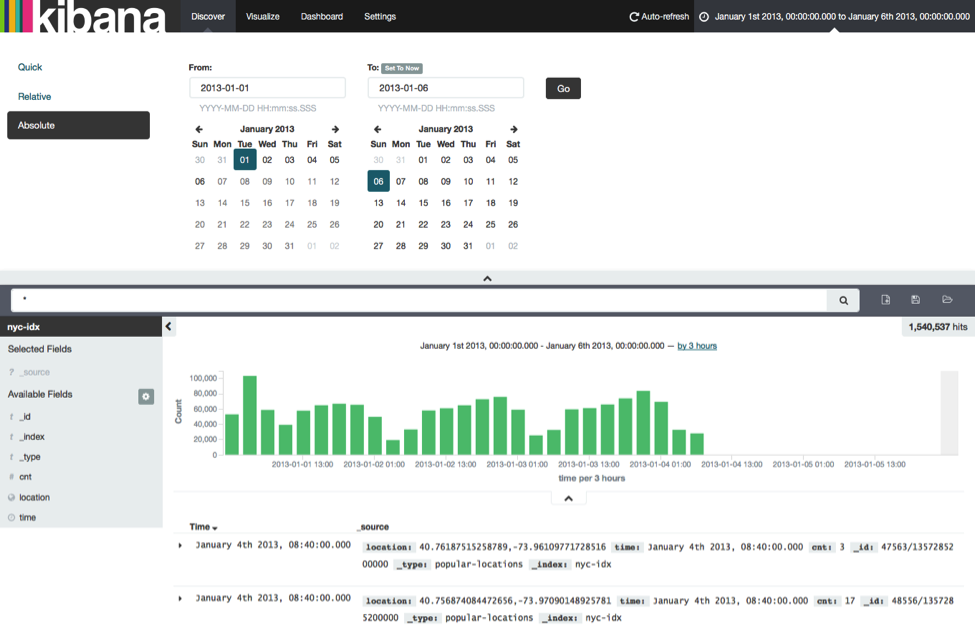
First click on the “Discover” button at the top of the page. You will find that Kibana tells you “No results found”.
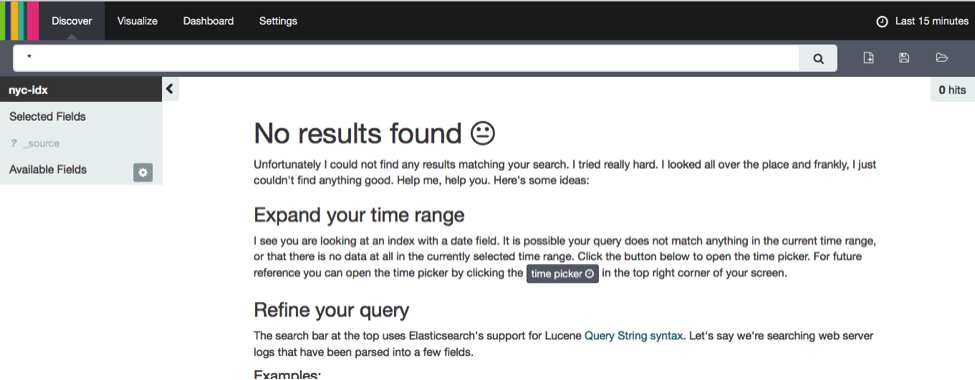
This is because Kibana restricts time-based events by default to the last 15 minutes. Since our taxi ride data stream starts on January, 1st 2013, we need to adapt the time range that is considered by Kibana. This is done by clicking on the label “Last 15 Minutes” in the top right corner and entering an absolute time range starting at 2013-01-01 and ending at 2013-01-06.
We have told Kibana where our data is and the valid time range and can continue to visualize the data. For example we can visualize the arrival counts on a map. Click on the “Visualize” button at the top of the page, select “Tile map”, and click on “From a new search”.
See the following screenshot for the tile map configuration (left-hand side).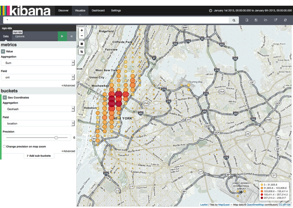
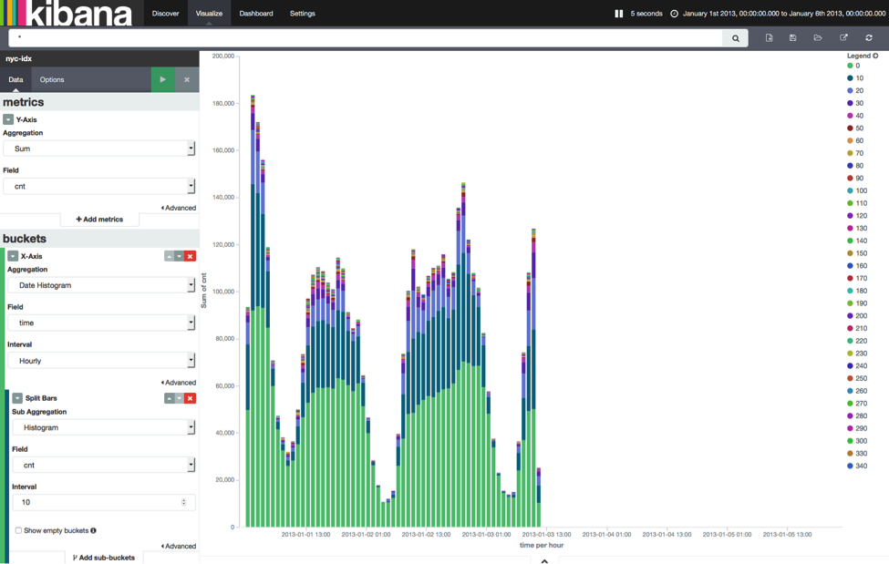
Another interesting visualization is to plot the number of arriving passengers over time. Click on “Visualize” at the top, select “Vertical bar chart”, and select “From a new search”. Again, have a look at the following screenshot for an example for how to configure the chart.
Kibana offers many more chart types and visualization options which are out of the scope of this post. You can easily play around with this setup, explore Kibana’s features, and implement your own Flink DataStream programs to analyze taxi rides in New York City.
We’re done and hope you had some fun
In this blog post we demonstrated how to build a real-time dashboard application with Apache Flink, Elasticsearch, and Kibana. By supporting event-time processing, Apache Flink is able to produce meaningful and consistent results even for historic data or in environments where events arrive out-of-order. The expressive DataStream API with flexible window semantics results in significantly less custom application logic compared to other open source stream processing solutions. Finally, connecting Flink with Elasticsearch and visualizing the real-time data with Kibana is just a matter of a few minutes. We hope you enjoyed running our demo application and had fun playing around with the code.
Fabian Hueske is a PMC member of Apache Flink. He is contributing to Flink  since its earliest days when it started as research project as part of his PhD studies at TU Berlin. Fabian did internships with IBM Research, SAP Research, and Microsoft Research and is a co-founder of data Artisans, a Berlin-based start-up devoted to foster Apache Flink. He is interested in distributed data processing and query optimization.
关于macos – go build runtime:darwin / amd64必须使用make.bash进行引导的介绍现已完结,谢谢您的耐心阅读,如果想了解更多关于bash – 安装make命令没有make(mac os 10.5)、Build caffe using qmake (ubuntu&windows)、Building an AI-powered Battlesnake with reinforcement learning on Amazon SageMaker、Building real-time dashboard applications with Apache Flink, Elasticsearch, and Kibana的相关知识,请在本站寻找。
本文标签:


