在本文中，我们将详细介绍多种方法决Win10系统上缺少Wi-Fi图标[COMPLETEGUIDE的各个方面，并为您提供关于win10缺少无线网卡驱动的相关解答，同时，我们也将为您带来关于Complet

在本文中，我们将详细介绍多种方法决Win10系统上缺少Wi-Fi图标[COMPLETE GUIDE的各个方面，并为您提供关于win10缺少无线网卡驱动的相关解答，同时，我们也将为您带来关于Complete Guide to Parameter Tuning in XGBoost (with codes in Python)、gulp遇到错误:The following tasks did not complete: default Did you forget to signal async completion?、Win10 WiFi不见了怎么恢复？Win10 WiFi图标不见了解决方法、win10wifi图标不见了的有用知识。

• 多种方法决Win10系统上缺少Wi-Fi图标[COMPLETE GUIDE（win10缺少无线网卡驱动）
• Complete Guide to Parameter Tuning in XGBoost (with codes in Python)
• gulp遇到错误:The following tasks did not complete: default Did you forget to signal async completion?
• Win10 WiFi不见了怎么恢复？Win10 WiFi图标不见了解决方法
• win10wifi图标不见了

多种方法决Win10系统上缺少Wi-Fi图标[COMPLETE GUIDE（win10缺少无线网卡驱动）

多种方法决Win10系统上缺少Wi-Fi图标[COMPLETE GUIDE]

我们许多人使用无线连接访问Internet ，但是Win10系统用户报告了Wi-Fi的异常问题。根据他们的说法，Win10系统中缺少Wi-Fi图标，所以让我们看看如何解决这个小问题。

如果Win10系统上的Wi-Fi图标丢失，该怎么办?

解决方案1 –重新安装无线适配器驱动程序

要解决此问题，您需要重新安装无线适配器驱动程序。为此，请首先为您的设备下载最新的无线适配器驱动程序。

之后，您需要按照以下步骤卸载当前安装的驱动程序：

1.按Windows键+ X打开“ 高级用户菜单”，然后从列表中选择“ 设备管理器 ”。

2.找到您的无线适配器，右键单击它，然后从菜单中选择“ 卸载 ”。

3.如果可用，请选择“ 删除该设备的驱动程序软件”，然后单击“ 确定”。

4.完成之后，重新启动 PC。

当您的PC重新启动时，Win10系统将自动安装默认驱动程序。如果默认驱动程序无法正常运行，请尝试安装已经下载的无线适配器驱动程序。

重新安装驱动程序后，Wi-Fi图标应再次出现。

●自动更新驱动程序(建议)

卸载驱动程序后，建议您自动重新安装/更新它们。手动下载和安装驱动程序的过程可能会导致安装错误的驱动程序，可能会导致系统严重故障。

在Windows计算机上更新驱动程序的更安全，更轻松的方法是使用自动工具。我们强烈建议使用DriverFix 工具。

它会自动识别计算机上的每个设备，并将其与来自广泛在线数据库的最新驱动程序版本进行匹配。然后，可以分批或一次更新驱动程序，而无需用户在此过程中做出任何复杂的决定。

下面是它的工作原理：

1.下载并安装DriverFix

2.安装后，该程序将快速扫描并识别过期或丢失的Windows驱动程序。

DriverFix将您的PC与它的1800万Windows驱动程序的Cloud数据库进行比较，并建议适当的更新。您需要做的就是等待扫描完成。

3.扫描完成后，您将获得一份完整报告，说明在PC上发现的过时驱动程序。查看列表，查看是否要单独更新或每个驱动程序一次更新。要一次更新一个驱动程序，请单击驱动程序名称旁边的“更新”链接。或只需单击“全部更新”按钮即可自动安装所有建议的更新。

注意：一些驱动程序需要分多个步骤安装，因此您必须多次单击“更新”按钮，直到安装了所有驱动程序。

免责声明：此工具的某些功能不是免费的。

________________________________________

解决方案2 –关闭Wi-Fi Sense

根据用户的说法，Wi-Fi Sense可能会导致Win10系统中缺少Wi-Fi图标，但是您可以通过禁用Wi-Fi Sense轻松解决此问题。为此，您需要按照以下步骤操作：

1.打开“ 设置”应用，然后转到“ 网络和Internet”。

2.转到Wi-Fi标签，然后点击管理Wi-Fi设置。

3.找到Wi-Fi Sense并将其关闭。

之后，重新启动PC并检查问题是否已解决。

解决方案3 –更改系统图标设置

有时由于系统图标设置的缘故，您的Wi-Fi图标可能会丢失。使用系统图标设置，您可以选择哪些图标将出现在任务栏上，因此请确保启用了网络图标。

为此，请按照下列步骤操作：

1.打开设置应用程序，然后转到系统。

2.导航到“ 通知和操作”选项卡，然后单击“ 打开或关闭系统图标”。

3.找到“ 网络”图标，并确保其已打开。如果不是，请重新打开。

4.返回并单击选择出现在任务栏上的图标。

5.查找“ 网络”图标，并确保将其设置为“ 开”。

之后，Wi-Fi图标应始终出现在任务栏中。

如果Win10系统桌面上缺少多个图标，请查看本指南以将其找回。

解决方案4 –确保您的无线适配器出现在设备管理器中

如果缺少Wi-Fi图标，则需要检查无线网络适配器是否出现在设备管理器中。为此，请按照下列步骤操作：

打开设备管理器。

当设备管理器打开时，单击硬件改动按钮扫描。

这样做之后，您的无线网络适配器应与Wi-Fi图标一起出现。

一些用户还建议从设备管理器中删除WAN Miniport适配器，因此您可能也想尝试一下。

解决方案5 –确保关闭飞行模式

根据用户，如果打开飞行模式会出现此问题，所以请务必检查飞行模式的状态。要关闭飞行模式，请执行以下操作：

1.打开行动中心。

2.找到飞行模式图标，然后单击以关闭飞行模式。

或者，您可以按照以下步骤从“设置”应用中关闭飞行模式：

1..打开“ 设置”应用，然后转到“ 网络和Internet”部分。

2.选择飞行模式选项卡，然后找到飞行模式部分。确保将“ 关闭所有无线通信”设置为“ 关闭”以禁用飞行模式。

飞行模式将停止所有无线通信，因此，如果缺少Wi-Fi图标，请确保检查飞行模式是否未打开。

如果您遇到任何飞行模式错误，建议您阅读本文。

解决方案6 –重新启动资源管理器

用户建议的一种解决方法是重新启动Windows资源管理器进程。由于某些未知原因，Win10系统上缺少Wi-Fi图标，但重新启动Windows资源管理器后，此问题已解决。

要重新启动Windows资源管理器，请执行以下操作：

1.通过按Ctrl + Shift + Esc打开任务管理器。

2.当任务管理器打开，找到Windows资源管理器进程，右键单击它并选择重新启动。

3.Windows资源管理器重新启动后，应显示Wi-Fi图标。

或者，您也可以从菜单中选择“结束任务”以结束Windows资源管理器进程。如果决定结束Windows资源管理器进程，则需要按照以下步骤手动重新启动它：

1.在任务管理器中，选择“ 文件”“运行新任务”。

2.输入资源管理器，然后按Enter或单击“ 确定”。

解决方案7 –编辑组策略

根据用户，您可以仅通过编辑组策略来启用Wi-Fi图标。为此，请按照下列步骤操作：

1.按Windows键+ R并输入gpedit.msc。按Enter或单击确定。

2.组策略编辑器现在将打开。在左窗格中，导航到“ 用户配置”“管理模板”“开始菜单”和“任务栏”。

3.在右窗格中找到“ 删除网络图标”选项，然后双击它。

4.选择禁用选项，然后单击应用和确定以保存更改。

5.关闭组策略编辑器，然后重新启动 PC。

解决方案8 –尝试禁用网络连接

如果缺少Wi-Fi图标，则可以通过禁用和启用无线网络连接来解决此问题。为此，请按照下列步骤操作：

1.按Windows键+ X，然后从菜单中选择“ 网络连接 ”。

2.当“ 网络连接”窗口打开时，右键单击您的无线网络，然后从菜单中选择“ 禁用 ”。

3.重复相同的步骤，但是这次从菜单中选择“ 启用 ”。

重新启用无线网络连接后，Wi-Fi图标应出现在任务栏上。

解决方案9 –执行完全关机

根据您的电源设置，当您按下电源按钮时，Win10系统可能不会完全关闭，但是您可以使用命令提示符关闭PC。为此，请按照下列步骤操作：

1.按Windows键+ X，然后从菜单中选择命令提示符(Admin)。

2.当命令提示符打开时，输入shutdown / p并按Enter。

您的电脑现在将完全关闭。系统重新启动后，应显示Wi-Fi图标。

解决方案10 –检查Wi-Fi图标是否隐藏

有时，Wi-Fi图标可能隐藏在任务栏上。要显示所有图标，请执行以下操作：

1.按右下角的顶部箭头显示隐藏的图标。

2.如果有可用的Wi-Fi图标，只需将其拖到任务栏，它应永久停留在该位置。

解决方案11-运行Internet故障排除程序

即使通常使用内置的Internet故障排除程序来解决连接问题，一些用户也确认它可以帮助他们解决丢失的Wi-Fi问题。

因此，请转至设置更新和安全疑难解答选择并运行Internet疑难解答。按照屏幕上的说明完成扫描，然后重新启动计算机。

解决方案12 –干净启动计算机

如果问题仍然存在，请执行干净启动。这样，您的Win10系统计算机将使用最少的驱动程序启动。如果缺少的Wi-Fi图标问题是由不兼容的驱动程序问题触发的，则此替代方法应可帮助您解决问题。

以下是要遵循的步骤：

1.键入系统配置 在搜索框中点击Enter

2.在“ 服务”选项卡上，选择“ 隐藏所有Microsoft服务”复选框，然后单击“ 全部禁用”。

3.在“ 启动” 选项卡上，单击“ 打开任务管理器”。

4.在“ 任务管理器”中 的“ 启动” 选项卡上，选择所有项目，然后单击“ 禁用”。

5.关闭任务管理器。

6. 在启动 的选项卡系统配置 对话框单击 OK 重新启动计算机检查Wi-Fi图标现在是可见的。

解决方案13 –创建一个新的用户配置文件

如果此Wi-Fi图标问题是由损坏的用户配置文件触发的，则您需要创建一个新的用户配置文件，并检查问题是否仍然存在于新的配置文件上。

以下是要遵循的步骤：

1.转到开始设置帐户家庭和其他人

2.选择“将其他人添加到此PC”

3.输入用户名，密码，密码提示单击下一步。

如果您的用户个人资料已损坏，则可以通过以下最佳方法快速轻松地对其进行修复。

Win10系统上缺少Wi-Fi图标不是主要问题，但是某些用户更喜欢在其任务栏上具有Wi-Fi图标。如果您遇到此问题，请确保尝试使用本文提供的一些解决方案。

Complete Guide to Parameter Tuning in XGBoost (with codes in Python)

Introduction

If things don’t go your way in predictive modeling, use XGboost.  XGBoost algorithm has become the ultimate weapon of many data scientist. It’s a highly sophisticated algorithm, powerful enough to deal with all sorts of irregularities of data.

Building a model using XGBoost is easy. But, improving the model using XGBoost is difficult (at least I struggled a lot). This algorithm uses multiple parameters. To improve the model, parameter tuning is must. It is very difficult to get answers to practical questions like – Which set of parameters you should tune ? What is the ideal value of these parameters to obtain optimal output ?

This article is best suited to people who are new to XGBoost. In this article, we’ll learn the art of parameter tuning along with some useful information about XGBoost. Also, we’ll practice this algorithm using a  data set in Python.

What should you know ?

XGBoost (eXtreme Gradient Boosting) is an advanced implementation of gradient boosting algorithm. Since I covered Gradient Boosting Machine in detail in my previous article – Complete Guide to Parameter Tuning in Gradient Boosting (GBM) in Python, I highly recommend going through that before reading further. It will help you bolster your understanding of boosting in general and parameter tuning for GBM.

Special Thanks: Personally, I would like to acknowledge the timeless support provided by Mr. Sudalai Rajkumar (aka SRK), currently AV Rank 2. This article wouldn’t be possible without his help. He is helping us guide thousands of data scientists. A big thanks to SRK!

Table of Contents

1. The XGBoost Advantage
2. Understanding XGBoost Parameters
3. Tuning Parameters (with Example)

1. The XGBoost Advantage

I’ve always admired the boosting capabilities that this algorithm infuses in a predictive model. When I explored more about its performance and science behind its high accuracy, I discovered many advantages:

1. Regularization:
   • Standard GBM implementation has no regularization like XGBoost, therefore it also helps to reduce overfitting.
   • In fact, XGBoost is also known as ‘regularized boosting‘ technique.
2. Parallel Processing:
   • XGBoost implements parallel processing and is blazingly faster as compared to GBM.
   • But hang on, we know that boosting is sequential process so how can it be parallelized? We know that each tree can be built only after the previous one, so what stops us from making a tree using all cores? I hope you get where I’m coming from. Check this link out to explore further.
   • XGBoost also supports implementation on Hadoop.
3. High Flexibility
   • XGBoost allow users to define custom optimization objectives and evaluation criteria.
   • This adds a whole new dimension to the model and there is no limit to what we can do.
4. Handling Missing Values
   • XGBoost has an in-built routine to handle missing values.
   • User is required to supply a different value than other observations and pass that as a parameter. XGBoost tries different things as it encounters a missing value on each node and learns which path to take for missing values in future.
5. Tree Pruning:
   • A GBM would stop splitting a node when it encounters a negative loss in the split. Thus it is more of a greedy algorithm.
   • XGBoost on the other hand make splits upto the max_depth specified and then start pruningthe tree backwards and remove splits beyond which there is no positive gain.
   • Another advantage is that sometimes a split of negative loss say -2 may be followed by a split of positive loss +10. GBM would stop as it encounters -2. But XGBoost will go deeper and it will see a combined effect of +8 of the split and keep both.
6. Built-in Cross-Validation
   • XGBoost allows user to run a cross-validation at each iteration of the boosting process and thus it is easy to get the exact optimum number of boosting iterations in a single run.
   • This is unlike GBM where we have to run a grid-search and only a limited values can be tested.
7. Continue on Existing Model
   • User can start training an XGBoost model from its last iteration of previous run. This can be of significant advantage in certain specific applications.
   • GBM implementation of sklearn also has this feature so they are even on this point.

I hope now you understand the sheer power XGBoost algorithm. Note that these are the points which I could muster. You know a few more? Feel free to drop a comment below and I will update the list.

Did I whet your appetite ? Good. You can refer to following web-pages for a deeper understanding:

• XGBoost Guide – Introduction to Boosted Trees
• Words from the Author of XGBoost [Video]

2. XGBoost Parameters

The overall parameters have been divided into 3 categories by XGBoost authors:

1. General Parameters: Guide the overall functioning
2. Booster Parameters: Guide the individual booster (tree/regression) at each step
3. Learning Task Parameters: Guide the optimization performed

I will give analogies to GBM here and highly recommend to read this article to learn from the very basics.

General Parameters

These define the overall functionality of XGBoost.

1. booster [default=gbtree]
   • Select the type of model to run at each iteration. It has 2 options:
     • gbtree: tree-based models
     • gblinear: linear models
2. silent [default=0]:
   • Silent mode is activated is set to 1, i.e. no running messages will be printed.
   • It’s generally good to keep it 0 as the messages might help in understanding the model.
3. nthread [default to maximum number of threads available if not set]
   • This is used for parallel processing and number of cores in the system should be entered
   • If you wish to run on all cores, value should not be entered and algorithm will detect automatically

There are 2 more parameters which are set automatically by XGBoost and you need not worry about them. Lets move on to Booster parameters.

Booster Parameters

Though there are 2 types of boosters, I’ll consider only tree booster here because it always outperforms the linear booster and thus the later is rarely used.

1. eta [default=0.3]
   • Analogous to learning rate in GBM
   • Makes the model more robust by shrinking the weights on each step
   • Typical final values to be used: 0.01-0.2
2. min_child_weight [default=1]
   • Defines the minimum sum of weights of all observations required in a child.
   • This is similar to min_child_leaf in GBM but not exactly. This refers to min “sum of weights” of observations while GBM has min “number of observations”.
   • Used to control over-fitting. Higher values prevent a model from learning relations which might be highly specific to the particular sample selected for a tree.
   • Too high values can lead to under-fitting hence, it should be tuned using CV.
3. max_depth [default=6]
   • The maximum depth of a tree, same as GBM.
   • Used to control over-fitting as higher depth will allow model to learn relations very specific to a particular sample.
   • Should be tuned using CV.
   • Typical values: 3-10
4. max_leaf_nodes
   • The maximum number of terminal nodes or leaves in a tree.
   • Can be defined in place of max_depth. Since binary trees are created, a depth of ‘n’ would produce a maximum of 2^n leaves.
   • If this is defined, GBM will ignore max_depth.
5. gamma [default=0]
   • A node is split only when the resulting split gives a positive reduction in the loss function. Gamma specifies the minimum loss reduction required to make a split.
   • Makes the algorithm conservative. The values can vary depending on the loss function and should be tuned.
6. max_delta_step [default=0]
   • In maximum delta step we allow each tree’s weight estimation to be. If the value is set to 0, it means there is no constraint. If it is set to a positive value, it can help making the update step more conservative.
   • Usually this parameter is not needed, but it might help in logistic regression when class is extremely imbalanced.
   • This is generally not used but you can explore further if you wish.
7. subsample [default=1]
   • Same as the subsample of GBM. Denotes the fraction of observations to be randomly samples for each tree.
   • Lower values make the algorithm more conservative and prevents overfitting but too small values might lead to under-fitting.
   • Typical values: 0.5-1
8. colsample_bytree [default=1]
   • Similar to max_features in GBM. Denotes the fraction of columns to be randomly samples for each tree.
   • Typical values: 0.5-1
9. colsample_bylevel [default=1]
   • Denotes the subsample ratio of columns for each split, in each level.
   • I don’t use this often because subsample and colsample_bytree will do the job for you. but you can explore further if you feel so.
10. lambda [default=1]
    • L2 regularization term on weights (analogous to Ridge regression)
    • This used to handle the regularization part of XGBoost. Though many data scientists don’t use it often, it should be explored to reduce overfitting.
11. alpha [default=0]
    • L1 regularization term on weight (analogous to Lasso regression)
    • Can be used in case of very high dimensionality so that the algorithm runs faster when implemented
12. scale_pos_weight [default=1]
    • A value greater than 0 should be used in case of high class imbalance as it helps in faster convergence.

Learning Task Parameters

These parameters are used to define the optimization objective the metric to be calculated at each step.

1. objective [default=reg:linear]
   • This defines the loss function to be minimized. Mostly used values are:
     • binary:logistic –logistic regression for binary classification, returns predicted probability (not class)
     • multi:softmax –multiclass classification using the softmax objective, returns predicted class (not probabilities)
       • you also need to set an additional num_class (number of classes) parameter defining the number of unique classes
     • multi:softprob –same as softmax, but returns predicted probability of each data point belonging to each class.
2. eval_metric [ default according to objective ]
   • The metric to be used for validation data.
   • The default values are rmse for regression and error for classification.
   • Typical values are:
     • rmse – root mean square error
     • mae – mean absolute error
     • logloss – negative log-likelihood
     • error – Binary classification error rate (0.5 threshold)
     • merror – Multiclass classification error rate
     • mlogloss – Multiclass logloss
     • auc: Area under the curve
3. seed [default=0]
   • The random number seed.
   • Can be used for generating reproducible results and also for parameter tuning.

If you’ve been using Scikit-Learn till now, these parameter names might not look familiar. A good news is that xgboost module in python has an sklearn wrapper called XGBClassifier. It uses sklearn style naming convention. The parameters names which will change are:

1. eta –> learning_rate
2. lambda –> reg_lambda
3. alpha –> reg_alpha

You must be wondering that we have defined everything except something similar to the “n_estimators” parameter in GBM. Well this exists as a parameter in XGBClassifier. However, it has to be passed as “num_boosting_rounds” while calling the fit function in the standard xgboost implementation.

I recommend you to go through the following parts of xgboost guide to better understand the parameters and codes:

1. XGBoost Parameters (official guide)
2. XGBoost Demo Codes (xgboost GitHub repository)
3. Python API Reference (official guide)

3. Parameter Tuning with Example

We will take the data set from Data Hackathon 3.x AV hackathon, same as that taken in the GBM article. The details of the problem can be found on the competition page. You can download the data set from here. I have performed the following steps:

1. City variable dropped because of too many categories
2. DOB converted to Age | DOB dropped
3. EMI_Loan_Submitted_Missing created which is 1 if EMI_Loan_Submitted was missing else 0 | Original variable EMI_Loan_Submitted dropped
4. EmployerName dropped because of too many categories
5. Existing_EMI imputed with 0 (median) since only 111 values were missing
6. Interest_Rate_Missing created which is 1 if Interest_Rate was missing else 0 | Original variable Interest_Rate dropped
7. Lead_Creation_Date dropped because made little intuitive impact on outcome
8. Loan_Amount_Applied, Loan_Tenure_Applied imputed with median values
9. Loan_Amount_Submitted_Missing created which is 1 if Loan_Amount_Submitted was missing else 0 | Original variable Loan_Amount_Submitted dropped
10. Loan_Tenure_Submitted_Missing created which is 1 if Loan_Tenure_Submitted was missing else 0 | Original variable Loan_Tenure_Submitted dropped
11. LoggedIn, Salary_Account dropped
12. Processing_Fee_Missing created which is 1 if Processing_Fee was missing else 0 | Original variable Processing_Fee dropped
13. Source – top 2 kept as is and all others combined into different category
14. Numerical and One-Hot-Coding performed

For those who have the original data from competition, you can check out these steps from the data_preparation iPython notebook in the repository.

Lets start by importing the required libraries and loading the data:

#Import libraries:
import pandas as pd
import numpy as np
import xgboost as xgb
from xgboost.sklearn import XGBClassifier
from sklearn import cross_validation, metrics   #Additional scklearn functions
from sklearn.grid_search import GridSearchCV   #Perforing grid search

import matplotlib.pylab as plt
%matplotlib inline
from matplotlib.pylab import rcParams
rcParams[''figure.figsize''] = 12, 4

train = pd.read_csv(''train_modified.csv'')
target = ''Disbursed''
IDcol = ''ID''

Note that I have imported 2 forms of XGBoost:

1. xgb – this is the direct xgboost library. I will use a specific function “cv” from this library
2. XGBClassifier – this is an sklearn wrapper for XGBoost. This allows us to use sklearn’s Grid Search with parallel processing in the same way we did for GBM

Before proceeding further, lets define a function which will help us create XGBoost models and perform cross-validation. The best part is that you can take this function as it is and use it later for your own models.

def modelfit(alg, dtrain, predictors,useTrainCV=True, cv_folds=5, early_stopping_rounds=50):
    
    if useTrainCV:
        xgb_param = alg.get_xgb_params()
        xgtrain = xgb.DMatrix(dtrain[predictors].values, label=dtrain[target].values)
        cvresult = xgb.cv(xgb_param, xgtrain, num_boost_round=alg.get_params()[''n_estimators''], nfold=cv_folds,
            metrics=''auc'', early_stopping_rounds=early_stopping_rounds, show_progress=False)
        alg.set_params(n_estimators=cvresult.shape[0])
    
    #Fit the algorithm on the data
    alg.fit(dtrain[predictors], dtrain[''Disbursed''],eval_metric=''auc'')
        
    #Predict training set:
    dtrain_predictions = alg.predict(dtrain[predictors])
    dtrain_predprob = alg.predict_proba(dtrain[predictors])[:,1]
        
    #Print model report:
    print "\nModel Report"
    print "Accuracy : %.4g" % metrics.accuracy_score(dtrain[''Disbursed''].values, dtrain_predictions)
    print "AUC Score (Train): %f" % metrics.roc_auc_score(dtrain[''Disbursed''], dtrain_predprob)
                    
    feat_imp = pd.Series(alg.booster().get_fscore()).sort_values(ascending=False)
    feat_imp.plot(kind=''bar'', title=''Feature Importances'')
    plt.ylabel(''Feature Importance Score'')

This code is slightly different from what I used for GBM. The focus of this article is to cover the concepts and not coding. Please feel free to drop a note in the comments if you find any challenges in understanding any part of it. Note that xgboost’s sklearn wrapper doesn’t have a “feature_importances” metric but a get_fscore() function which does the same job.

General Approach for Parameter Tuning

We will use an approach similar to that of GBM here. The various steps to be performed are:

1. Choose a relatively high learning rate. Generally a learning rate of 0.1 works but somewhere between 0.05 to 0.3 should work for different problems. Determine the optimum number of trees for this learning rate. XGBoost has a very useful function called as “cv” which performs cross-validation at each boosting iteration and thus returns the optimum number of trees required.
2. Tune tree-specific parameters ( max_depth, min_child_weight, gamma, subsample, colsample_bytree) for decided learning rate and number of trees. Note that we can choose different parameters to define a tree and I’ll take up an example here.
3. Tune regularization parameters (lambda, alpha) for xgboost which can help reduce model complexity and enhance performance.
4. Lower the learning rate and decide the optimal parameters .

Let us look at a more detailed step by step approach.

Step 1: Fix learning rate and number of estimators for tuning tree-based parameters

In order to decide on boosting parameters, we need to set some initial values of other parameters. Lets take the following values:

1. max_depth = 5 : This should be between 3-10. I’ve started with 5 but you can choose a different number as well. 4-6 can be good starting points.
2. min_child_weight = 1 : A smaller value is chosen because it is a highly imbalanced class problem and leaf nodes can have smaller size groups.
3. gamma = 0 : A smaller value like 0.1-0.2 can also be chosen for starting. This will anyways be tuned later.
4. subsample, colsample_bytree = 0.8 : This is a commonly used used start value. Typical values range between 0.5-0.9.
5. scale_pos_weight = 1: Because of high class imbalance.

Please note that all the above are just initial estimates and will be tuned later. Lets take the default learning rate of 0.1 here and check the optimum number of trees using cv function of xgboost. The function defined above will do it for us.

#Choose all predictors except target & IDcols
predictors = [x for x in train.columns if x not in [target, IDcol]]
xgb1 = XGBClassifier(
 learning_rate =0.1,
 n_estimators=1000,
 max_depth=5,
 min_child_weight=1,
 gamma=0,
 subsample=0.8,
 colsample_bytree=0.8,
 objective= ''binary:logistic'',
 nthread=4,
 scale_pos_weight=1,
 seed=27)
modelfit(xgb1, train, predictors)

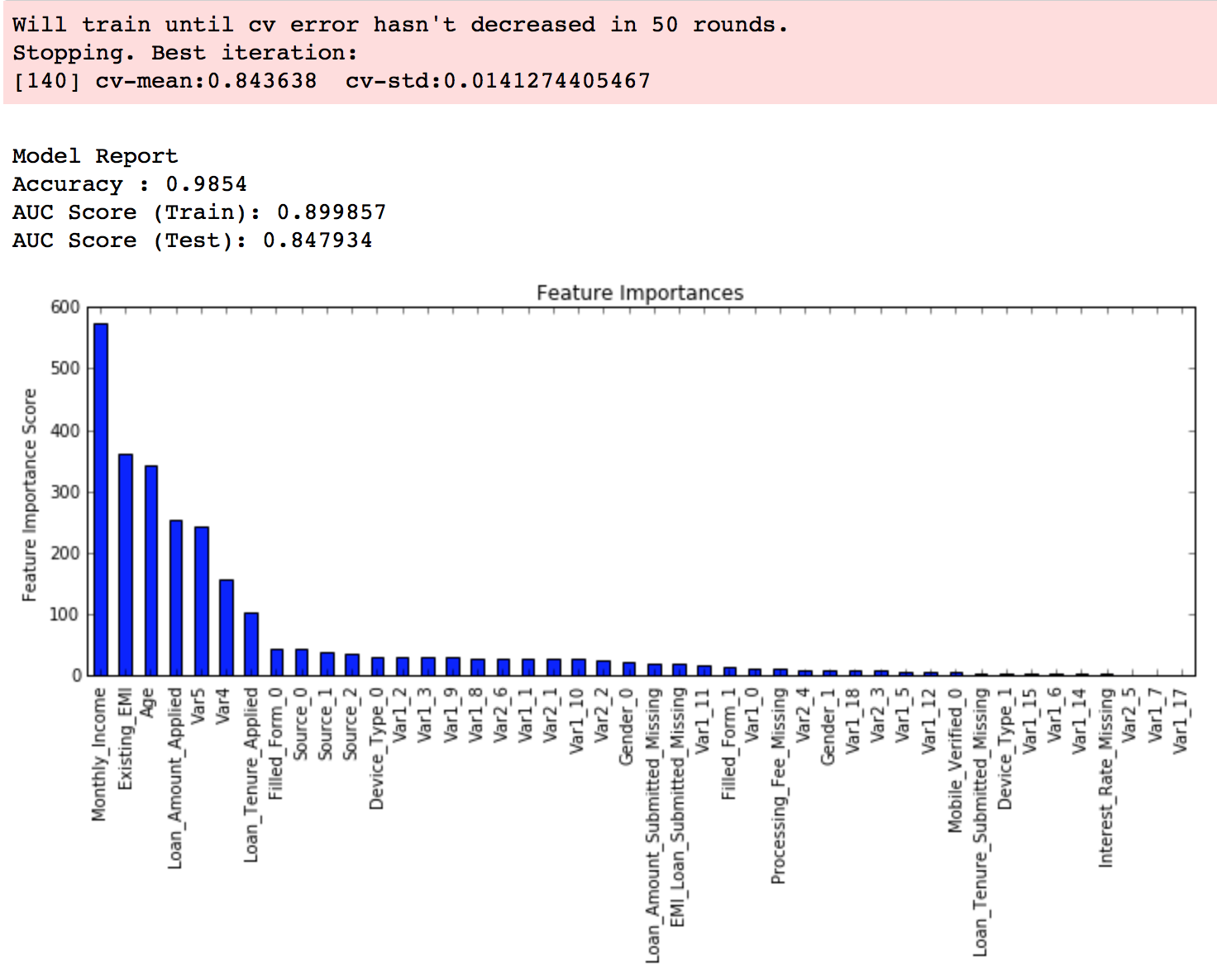
As you can see that here we got 140 as the optimal estimators for 0.1 learning rate. Note that this value might be too high for you depending on the power of your system. In that case you can increase the learning rate and re-run the command to get the reduced number of estimators.

Note: You will see the test AUC as “AUC Score (Test)” in the outputs here. But this would not appear if you try to run the command on your system as the data is not made public. It’s provided here just for reference. The part of the code which generates this output has been removed here.

Step 2: Tune max_depth and min_child_weight

We tune these first as they will have the highest impact on model outcome. To start with, let’s set wider ranges and then we will perform another iteration for smaller ranges.

Important Note: I’ll be doing some heavy-duty grid searched in this section which can take 15-30 mins or even more time to run depending on your system. You can vary the number of values you are testing based on what your system can handle.

param_test1 = {
 ''max_depth'':range(3,10,2),
 ''min_child_weight'':range(1,6,2)
}
gsearch1 = GridSearchCV(estimator = XGBClassifier( learning_rate =0.1, n_estimators=140, max_depth=5,
 min_child_weight=1, gamma=0, subsample=0.8, colsample_bytree=0.8,
 objective= ''binary:logistic'', nthread=4, scale_pos_weight=1, seed=27), 
 param_grid = param_test1, scoring=''roc_auc'',n_jobs=4,iid=False, cv=5)
gsearch1.fit(train[predictors],train[target])
gsearch1.grid_scores_, gsearch1.best_params_, gsearch1.best_score_

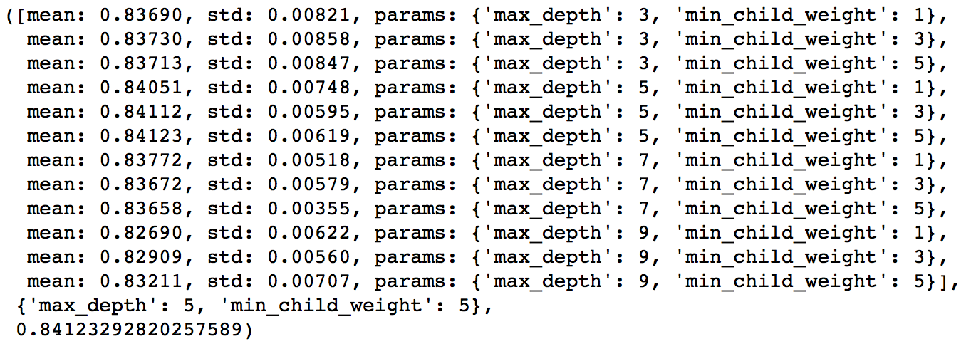
Here, we have run 12 combinations with wider intervals between values. The ideal values are 5 for max_depth and 5 for min_child_weight. Lets go one step deeper and look for optimum values. We’ll search for values 1 above and below the optimum values because we took an interval of two.

param_test2 = {
 ''max_depth'':[4,5,6],
 ''min_child_weight'':[4,5,6]
}
gsearch2 = GridSearchCV(estimator = XGBClassifier( learning_rate=0.1, n_estimators=140, max_depth=5,
 min_child_weight=2, gamma=0, subsample=0.8, colsample_bytree=0.8,
 objective= ''binary:logistic'', nthread=4, scale_pos_weight=1,seed=27), 
 param_grid = param_test2, scoring=''roc_auc'',n_jobs=4,iid=False, cv=5)
gsearch2.fit(train[predictors],train[target])
gsearch2.grid_scores_, gsearch2.best_params_, gsearch2.best_score_

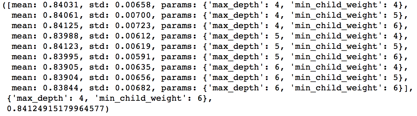
Here, we get the optimum values as 4 for max_depth and 6 for min_child_weight. Also, we can see the CV score increasing slightly. Note that as the model performance increases, it becomes exponentially difficult to achieve even marginal gains in performance. You would have noticed that here we got 6 as optimum value for min_child_weight but we haven’t tried values more than 6. We can do that as follow:.

param_test2b = {
 ''min_child_weight'':[6,8,10,12]
}
gsearch2b = GridSearchCV(estimator = XGBClassifier( learning_rate=0.1, n_estimators=140, max_depth=4,
 min_child_weight=2, gamma=0, subsample=0.8, colsample_bytree=0.8,
 objective= ''binary:logistic'', nthread=4, scale_pos_weight=1,seed=27), 
 param_grid = param_test2b, scoring=''roc_auc'',n_jobs=4,iid=False, cv=5)
gsearch2b.fit(train[predictors],train[target])

modelfit(gsearch3.best_estimator_, train, predictors)
gsearch2b.grid_scores_, gsearch2b.best_params_, gsearch2b.best_score_

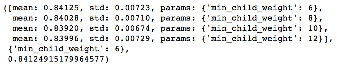
We see 6 as the optimal value.

Step 3: Tune gamma

Now lets tune gamma value using the parameters already tuned above. Gamma can take various values but I’ll check for 5 values here. You can go into more precise values as.

param_test3 = {
 ''gamma'':[i/10.0 for i in range(0,5)]
}
gsearch3 = GridSearchCV(estimator = XGBClassifier( learning_rate =0.1, n_estimators=140, max_depth=4,
 min_child_weight=6, gamma=0, subsample=0.8, colsample_bytree=0.8,
 objective= ''binary:logistic'', nthread=4, scale_pos_weight=1,seed=27), 
 param_grid = param_test3, scoring=''roc_auc'',n_jobs=4,iid=False, cv=5)
gsearch3.fit(train[predictors],train[target])
gsearch3.grid_scores_, gsearch3.best_params_, gsearch3.best_score_

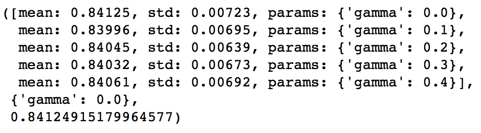
This shows that our original value of gamma, i.e. 0 is the optimum one. Before proceeding, a good idea would be to re-calibrate the number of boosting rounds for the updated parameters.

xgb2 = XGBClassifier(
 learning_rate =0.1,
 n_estimators=1000,
 max_depth=4,
 min_child_weight=6,
 gamma=0,
 subsample=0.8,
 colsample_bytree=0.8,
 objective= ''binary:logistic'',
 nthread=4,
 scale_pos_weight=1,
 seed=27)
modelfit(xgb2, train, predictors)

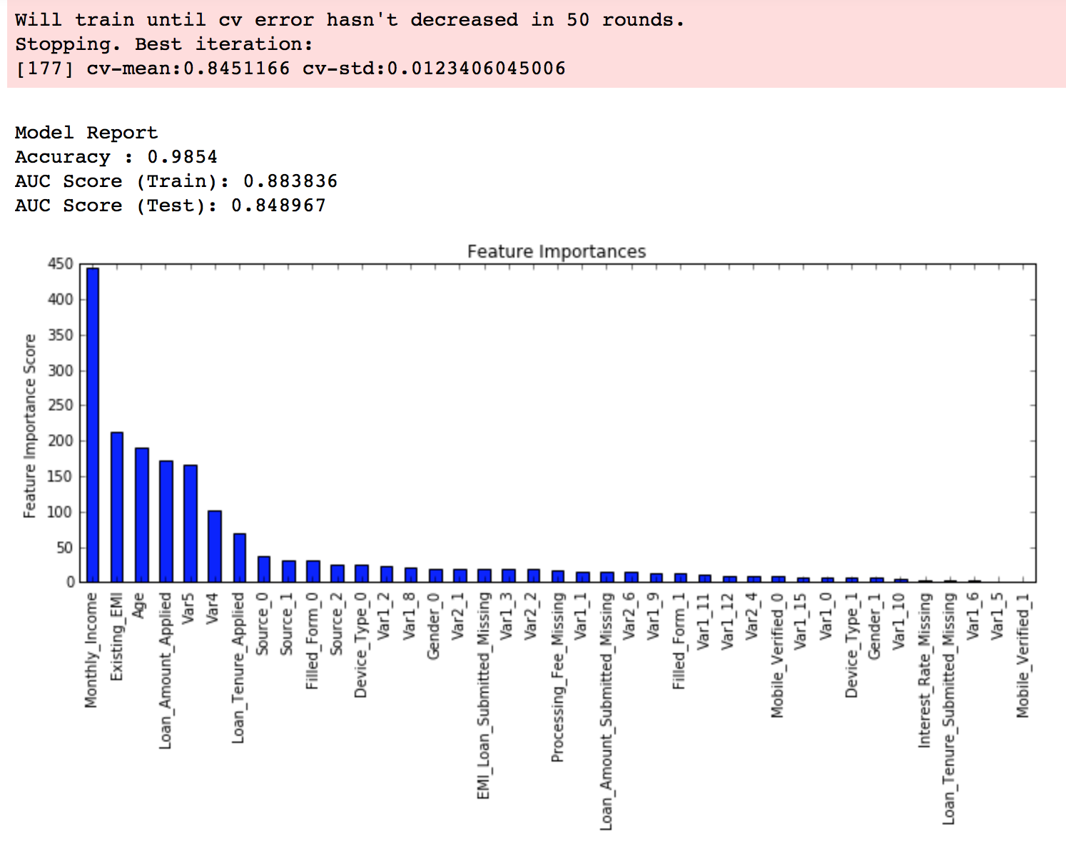Here, we can see the improvement in score. So the final parameters are:

• max_depth: 4
• min_child_weight: 6
• gamma: 0

Step 4: Tune subsample and colsample_bytree

The next step would be try different subsample and colsample_bytree values. Lets do this in 2 stages as well and take values 0.6,0.7,0.8,0.9 for both to start with.

param_test4 = {
 ''subsample'':[i/10.0 for i in range(6,10)],
 ''colsample_bytree'':[i/10.0 for i in range(6,10)]
}
gsearch4 = GridSearchCV(estimator = XGBClassifier( learning_rate =0.1, n_estimators=177, max_depth=4,
 min_child_weight=6, gamma=0, subsample=0.8, colsample_bytree=0.8,
 objective= ''binary:logistic'', nthread=4, scale_pos_weight=1,seed=27), 
 param_grid = param_test4, scoring=''roc_auc'',n_jobs=4,iid=False, cv=5)
gsearch4.fit(train[predictors],train[target])
gsearch4.grid_scores_, gsearch4.best_params_, gsearch4.best_score_

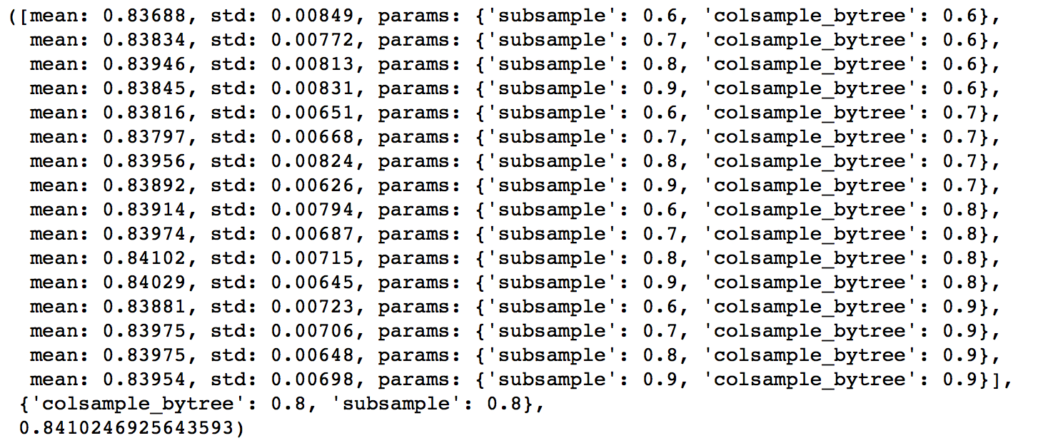
Here, we found 0.8 as the optimum value for both subsample and colsample_bytree. Now we should try values in 0.05 interval around these.

param_test5 = {
 ''subsample'':[i/100.0 for i in range(75,90,5)],
 ''colsample_bytree'':[i/100.0 for i in range(75,90,5)]
}
gsearch5 = GridSearchCV(estimator = XGBClassifier( learning_rate =0.1, n_estimators=177, max_depth=4,
 min_child_weight=6, gamma=0, subsample=0.8, colsample_bytree=0.8,
 objective= ''binary:logistic'', nthread=4, scale_pos_weight=1,seed=27), 
 param_grid = param_test5, scoring=''roc_auc'',n_jobs=4,iid=False, cv=5)
gsearch5.fit(train[predictors],train[target])

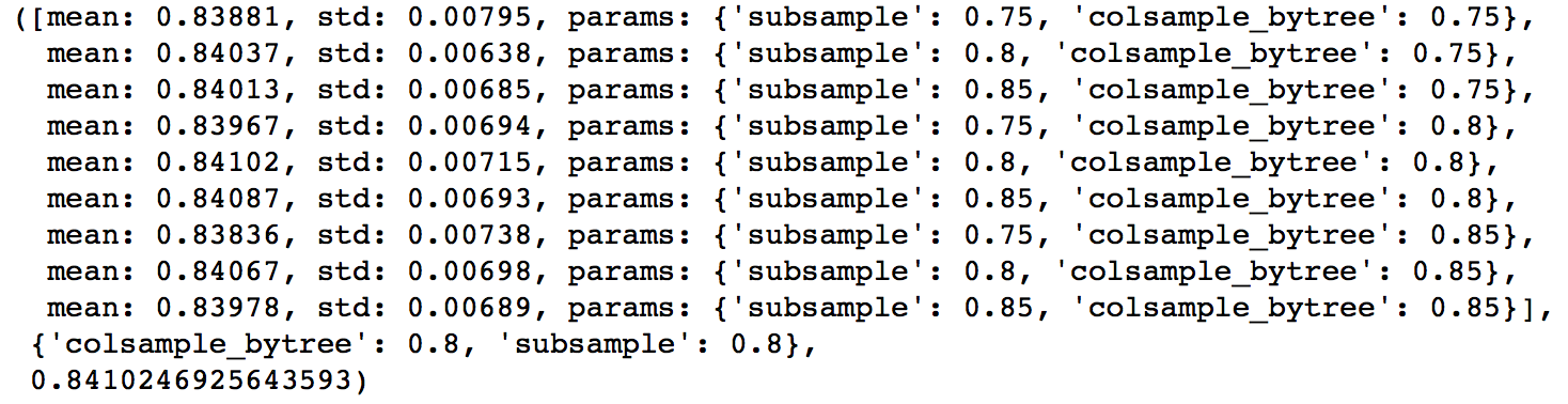
Again we got the same values as before. Thus the optimum values are:

• subsample: 0.8
• colsample_bytree: 0.8

Step 5: Tuning Regularization Parameters

Next step is to apply regularization to reduce overfitting. Though many people don’t use this parameters much as gamma provides a substantial way of controlling complexity. But we should always try it. I’ll tune ‘reg_alpha’ value here and leave it upto you to try different values of ‘reg_lambda’.

param_test6 = {
 ''reg_alpha'':[1e-5, 1e-2, 0.1, 1, 100]
}
gsearch6 = GridSearchCV(estimator = XGBClassifier( learning_rate =0.1, n_estimators=177, max_depth=4,
 min_child_weight=6, gamma=0.1, subsample=0.8, colsample_bytree=0.8,
 objective= ''binary:logistic'', nthread=4, scale_pos_weight=1,seed=27), 
 param_grid = param_test6, scoring=''roc_auc'',n_jobs=4,iid=False, cv=5)
gsearch6.fit(train[predictors],train[target])
gsearch6.grid_scores_, gsearch6.best_params_, gsearch6.best_score_

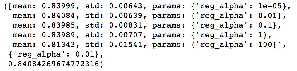
We can see that the CV score is less than the previous case. But the values tried are very widespread, we should try values closer to the optimum here (0.01) to see if we get something better.

param_test7 = {
 ''reg_alpha'':[0, 0.001, 0.005, 0.01, 0.05]
}
gsearch7 = GridSearchCV(estimator = XGBClassifier( learning_rate =0.1, n_estimators=177, max_depth=4,
 min_child_weight=6, gamma=0.1, subsample=0.8, colsample_bytree=0.8,
 objective= ''binary:logistic'', nthread=4, scale_pos_weight=1,seed=27), 
 param_grid = param_test7, scoring=''roc_auc'',n_jobs=4,iid=False, cv=5)
gsearch7.fit(train[predictors],train[target])
gsearch7.grid_scores_, gsearch7.best_params_, gsearch7.best_score_

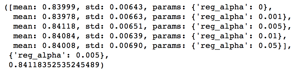
You can see that we got a better CV. Now we can apply this regularization in the model and look at the impact:

xgb3 = XGBClassifier(
 learning_rate =0.1,
 n_estimators=1000,
 max_depth=4,
 min_child_weight=6,
 gamma=0,
 subsample=0.8,
 colsample_bytree=0.8,
 reg_alpha=0.005,
 objective= ''binary:logistic'',
 nthread=4,
 scale_pos_weight=1,
 seed=27)
modelfit(xgb3, train, predictors)

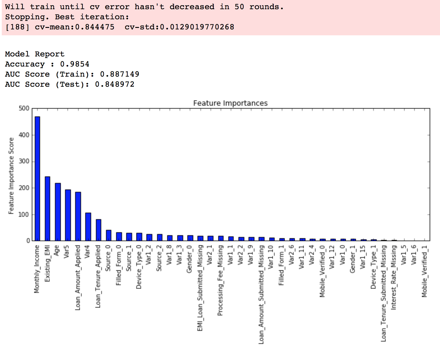
Again we can see slight improvement in the score.

Step 6: Reducing Learning Rate

Lastly, we should lower the learning rate and add more trees. Lets use the cv function of XGBoost to do the job again.

xgb4 = XGBClassifier(
 learning_rate =0.01,
 n_estimators=5000,
 max_depth=4,
 min_child_weight=6,
 gamma=0,
 subsample=0.8,
 colsample_bytree=0.8,
 reg_alpha=0.005,
 objective= ''binary:logistic'',
 nthread=4,
 scale_pos_weight=1,
 seed=27)
modelfit(xgb4, train, predictors)

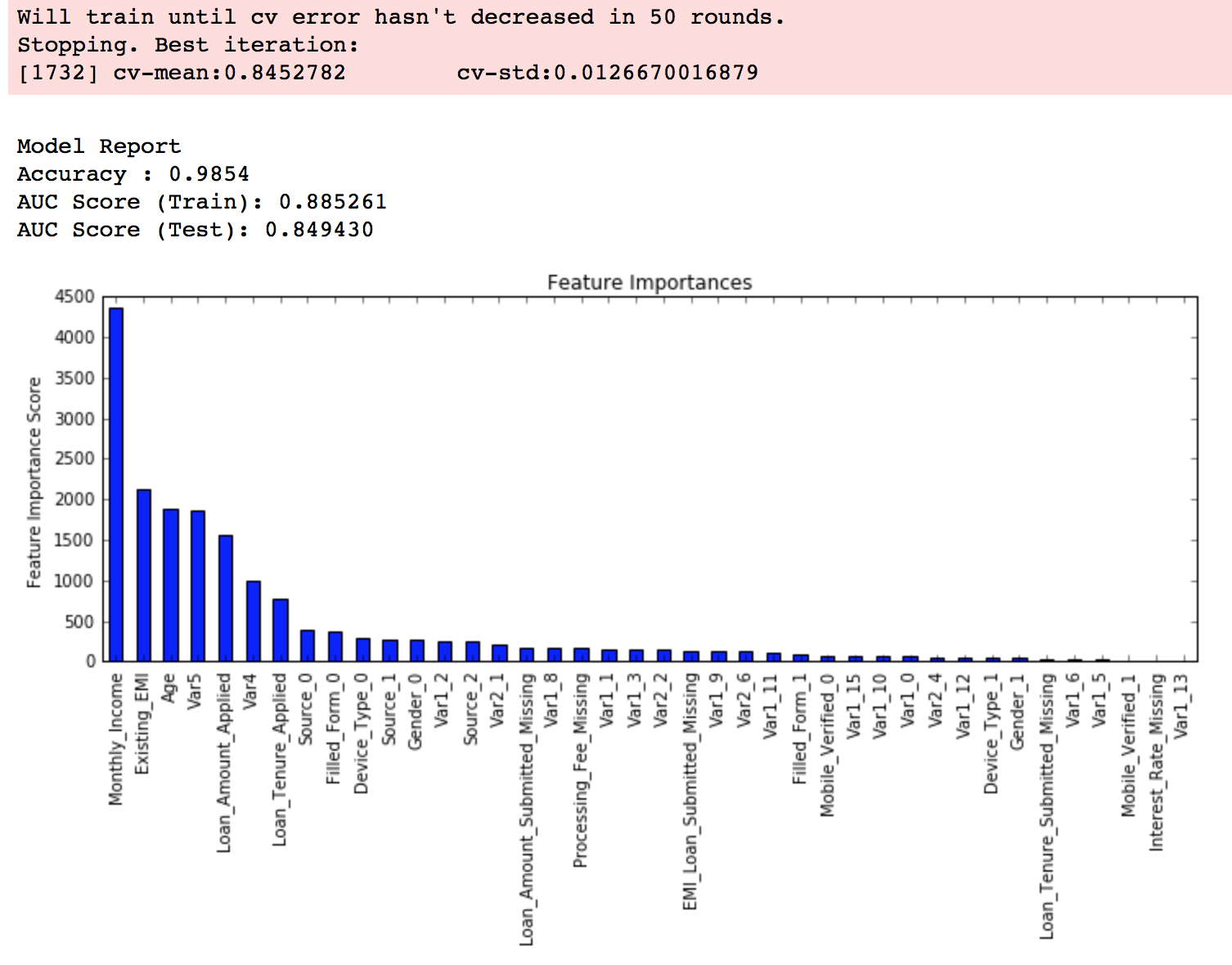
Now we can see a significant boost in performance and the effect of parameter tuning is clearer.

As we come to the end, I would like to share 2 key thoughts:

1. It is difficult to get a very big leap in performance by just using parameter tuning or slightly better models. The max score for GBM was 0.8487 while XGBoost gave 0.8494. This is a decent improvement but not something very substantial.
2. A significant jump can be obtained by other methods like feature engineering, creating ensemble of models, stacking, etc

You can also download the iPython notebook with all these model codes from my GitHub account. For codes in R, you can refer to this article.

End Notes

This article was based on developing a XGBoost model end-to-end. We started with discussing why XGBoost has superior performance over GBM which was followed by detailed discussion on thevarious parameters involved. We also defined a generic function which you can re-use for making models.

Finally, we discussed the general approach towards tackling a problem with XGBoost and also worked out the AV Data Hackathon 3.x problem through that approach.

I hope you found this useful and now you feel more confident to apply XGBoost in solving a data science problem. You can try this out in out upcoming hackathons.

Did you like this article? Would you like to share some other hacks which you implement while making XGBoost models? Please feel free to drop a note in the comments below and I’ll be glad to discuss.

You want to apply your analytical skills and test your potential? Then participate in our Hackathons and compete with Top Data Scientists from all over the world.

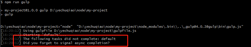
gulp遇到错误:The following tasks did not complete: default Did you forget to signal async completion?

运行之后会像下面一样报这个错误,因为事按着一个视频来写的,所以

 原本的gulpfile.js如下

const gulp = require(''gulp'')
gulp.task(''default'',()=>{
    // console.log(''default task'');
    gulp.src([''src/**/*''])
        .pipe(gulp.dest(''build''))
   
})

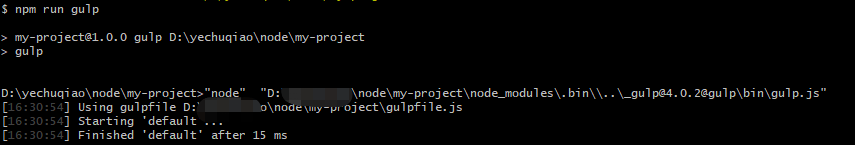
改成如下的形式就可以了

const gulp = require(''gulp'')
gulp.task(''default'',function(done){
    // console.log(''default task'');
    gulp.src([''src/**/*''])
        .pipe(gulp.dest(''build''))
        done()
})

运行之后

原因：因为gulp不再支持同步任务．因为同步任务常常会导致难以调试的细微错误，例如忘记从任务（task）中返回 stream。

当你看到 "Did you forget to signal async completion?" 警告时，说明你并未使用前面提到的返回方式。你需要使用 callback 或返回 stream、promise、event emitter、child process、observable 来解决此问题。具体详情请看API的异步执行

Win10 WiFi不见了怎么恢复？Win10 WiFi图标不见了解决方法

最近有看到很多用户反映自己的Win10笔记本电脑，WiFi图标不见了，导致无法连接网络，对日常工作很影响，那么怎么解决这个问题呢？下面一起来看看吧。

解决方法如下：

1、首先按下快捷键“win+r”打开运行，输入“service.msc”。

2、然后在服务列表中打开“WLAN autoconfig”在常规中找到“启动类型”，

将其改为自动，然后将服务状态改为“已停止”，点击启动。

3、在依次打开：

HKEY_LOCAL_MACHInesYstemCurrentControlSetServicesNdisuio

然后在右侧找到“displayname”，

4、然后右击“start”将数值数据改成2，点击确定。

5、之后按下快捷键“win+r”打开运行，输入cmd打开命令提示符。

6、最后输入“netsh winsock reset”重启即可。

以上就是win10系统wifi图标不见了解决方法的详细内容，希望可以帮助大家解决问题。

win10wifi图标不见了

进入win10系统操作之后，肯定会又很多的问题，最头疼的肯定就是wifi图标没了，导致没法连接无线网络，所以下面就提供了win10wifi图标不见了解决方法帮你们找到图标。

win10wifi图标不见了：

1、首先按下快捷键“win+r”打开运行，输入“service.msc”。

2、然后在服务列表中打开“WLAN autoconfig”在常规中找到“启动类型”，

将其改为自动，然后将服务状态改为“已停止”，点击启动。

3、在依次打开：

HKEY_LOCAL_MACHInesYstemCurrentControlSetServicesNdisuio

然后在右侧找到“displayname”，

4、然后右击“start”将数值数据改成2，点击确定。

5、之后按下快捷键“win+r”打开运行，输入cmd打开命令提示符。

6、最后输入“netsh winsock reset”重启即可。

今天关于多种方法决Win10系统上缺少Wi-Fi图标[COMPLETE GUIDE和win10缺少无线网卡驱动的讲解已经结束，谢谢您的阅读，如果想了解更多关于Complete Guide to Parameter Tuning in XGBoost (with codes in Python)、gulp遇到错误:The following tasks did not complete: default Did you forget to signal async completion?、Win10 WiFi不见了怎么恢复？Win10 WiFi图标不见了解决方法、win10wifi图标不见了的相关知识，请在本站搜索。