CS224d: Deep Learning for Natural Language Process

25-03-03 16

如果您对CS224d:DeepLearningforNaturalLanguageProcess感兴趣，那么本文将是一篇不错的选择，我们将为您详在本文中，您将会了解到关于CS224d:DeepLear

如果您对CS224d: Deep Learning for Natural Language Process感兴趣，那么本文将是一篇不错的选择，我们将为您详在本文中，您将会了解到关于CS224d: Deep Learning for Natural Language Process的详细内容，并且为您提供关于(转) Ensemble Methods for Deep Learning Neural Networks to Reduce Variance and Improve Performance、A Discriminative Feature Learning Approach for Deep Face Recognition、A Gentle Introduction to Transfer Learning for Deep Learning | 迁移学习、AN EMPIRICAL STUDY OF EXAMPLE FORGETTING DURING DEEP NEURAL NETWORK LEARNING 论文笔记的有价值信息。

本文目录一览：

CS224d: Deep Learning for Natural Language Process
(转) Ensemble Methods for Deep Learning Neural Networks to Reduce Variance and Improve Performance
A Discriminative Feature Learning Approach for Deep Face Recognition
A Gentle Introduction to Transfer Learning for Deep Learning | 迁移学习
AN EMPIRICAL STUDY OF EXAMPLE FORGETTING DURING DEEP NEURAL NETWORK LEARNING 论文笔记

CS224d: Deep Learning for Natural Language Process

Course Description

Teaching Assistants

Peng Qi

Course Notes (updated each week) Detailed Syllabus

Class Time and Location

Spring quarter (March - June, 2015).
Lecture: Monday, Wednesday 11:00-12:15
Location: TBD

Office Hours

Richard: Wed 12:45 - 2:00, Location: TBD
(for research and project discussions)
TAs: TBD

Grading Policy

Assignment #1: 15%
Assignment #2: 15%
Assignment #3: 15%
Midterm: 15%
Final Project: 40%

Course Discussions

Stanford students: Piazza (for Stanford students)
Online discussions: Reddit Group (for non-Stanford students)
Our Twitter account: @CS224d

Assignment Details

See the Assignment Page (coming soon) for more details on how to hand in your assignments.

Course Project Details

See the Project Page (coming soon) for more details on the course project.

Prerequisites

Proficiency in Python
All class assignments will be in Python (and use numpy). There is a tutorial here for those who aren''t as familiar with Python. If you have a lot of programming experience but in a different language (e.g. C/C++/Matlab/Javascript) you will probably be fine.
College Calculus, Linear Algebra (e.g. MATH 19 or 41, MATH 51)
You should be comfortable taking derivatives and understanding matrix vector operations and notation.
Basic Probability and Statistics (e.g. CS 109 or other stats course)
You should know basics of probabilities, gaussian distributions, mean, standard deviation, etc.
Equivalent knowledge of CS229 (Machine Learning)
We will be formulating cost functions, taking derivatives and performing optimization with gradient descent.

Knowledge of natural language processing (CS224N or CS224U)
We will discuss a lot of different tasks and you will appreciate the power of deep learning techniques even more if you know how much work had been done on these tasks and how related models have solved them.
Convex optimization
You may find some of the optimization tricks more intuitive with this background.
Knowledge of convolutional neural networks (CS231n)
The first problem set will probably be easier for you. We cannot assume you took this class so there will be ~3 lectures that overlap in content. You can use that time to dive deeper into some aspects.

FAQ

Is this the first time this class is offered?

Yes, this is an entirely new class designed to introduce students to deep learning for natural language processing. We will place a particular emphasis on Neural Networks, which are a class of deep learning models that have recently obtained improvements in many different NLP tasks.

Can I follow along from the outside?

We''d be happy if you join us! We plan to make the course materials widely available: The assignments, course notes and slides will be available online.We may provide videos. We won''t be able to give you course credit.

Can I take this course on credit/no cred basis?

Yes. Credit will be given to those who would have otherwise earned a C- or above.

Can I audit or sit in?

In general we are very open to sitting-in guests if you are a member of the Stanford community (registered student, staff, and/or faculty). Out of courtesy, we would appreciate that you first email us or talk to the instructor after the first class you attend.

Can I work in groups for the Final Project?

Yes, in groups of up to two people.

I have a question about the class. What is the best way to reach the course staff?

Stanford students please use an internal class forum on Piazza so that other students may benefit from your questions and our answers. If you have a personal matter, email us at the class mailing list cs224d-spr1415-staff@lists.stanford.edu.

Can I combine the Final Project with another course?

Yes, you may. There are a couple of courses concurrently offered with CS224d that are natural choices, such as CS224u (Natural Language Understanding, by Prof. Chris Potts and Bill MacCartney). If you are taking a related class, please speak to the instructors to receive permission to combine the Final Project assignments.

Natural language processing (NLP) is one of the most important technologies of the information age. Understanding complex language utterances is also a crucial part of artificial intelligence. Applications of NLP are everywhere because people communicate most everything in language: web search, advertisement, emails, customer service, language translation, radiology reports, etc. There are a large variety of underlying tasks and machine learning models powering NLP applications. Recently, deep learning approaches have obtained very high performance across many different NLP tasks. These models can often be trained with a single end-to-end model and do not require traditional, task-specific feature engineering. In this spring quarter course students will learn to implement, train, debug, visualize and invent their own neural network models. The course provides a deep excursion into cutting-edge research in deep learning applied to NLP. The final project will involve training a complex recurrent neural network and applying it to a large scale NLP problem. On the model side we will cover word vector representations, window-based neural networks, recurrent neural networks, long-short-term-memory models, recursive neural networks, convolutional neural networks as well as some very novel models involving a memory component. Through lectures and programming assignments students will learn the necessary engineering tricks for making neural networks work on practical problems.

Course Instructor

Richard Socher

(转) Ensemble Methods for Deep Learning Neural Networks to Reduce Variance and Improve Performance

Ensemble Methods for Deep Learning Neural Networks to Reduce Variance and Improve Performance

2018-12-19 13:02:45

This blog is copied from: https://machinelearningmastery.com/ensemble-methods-for-deep-learning-neural-networks/

Deep learning neural networks are nonlinear methods.

They offer increased flexibility and can scale in proportion to the amount of training data available. A downside of this flexibility is that they learn via a stochastic training algorithm which means that they are sensitive to the specifics of the training data and may find a different set of weights each time they are trained, which in turn produce different predictions.

Generally, this is referred to as neural networks having a high variance and it can be frustrating when trying to develop a final model to use for making predictions.

A successful approach to reducing the variance of neural network models is to train multiple models instead of a single model and to combine the predictions from these models. This is called ensemble learning and not only reduces the variance of predictions but also can result in predictions that are better than any single model.

In this post, you will discover methods for deep learning neural networks to reduce variance and improve prediction performance.

After reading this post, you will know:

Neural network models are nonlinear and have a high variance, which can be frustrating when preparing a final model for making predictions.
Ensemble learning combines the predictions from multiple neural network models to reduce the variance of predictions and reduce generalization error.
Techniques for ensemble learning can be grouped by the element that is varied, such as training data, the model, and how predictions are combined.

Let’s get started.

Ensemble Methods to Reduce Variance and Improve Performance of Deep Learning Neural Networks
Photo by University of San Francisco’s Performing Arts, some rights reserved.

Overview

This tutorial is divided into four parts; they are:

High Variance of Neural Network Models
Reduce Variance Using an Ensemble of Models
How to Ensemble Neural Network Models
Summary of Ensemble Techniques

High Variance of Neural Network Models

Training deep neural networks can be very computationally expensive.

Very deep networks trained on millions of examples may take days, weeks, and sometimes months to train.

Google’s baseline model […] was a deep convolutional neural network […] that had been trained for about six months using asynchronous stochastic gradient descent on a large number of cores.

— Distilling the Knowledge in a Neural Network, 2015.

After the investment of so much time and resources, there is no guarantee that the final model will have low generalization error, performing well on examples not seen during training.

… train many different candidate networks and then to select the best, […] and to discard the rest. There are two disadvantages with such an approach. First, all of the effort involved in training the remaining networks is wasted. Second, […] the network which had best performance on the validation set might not be the one with the best performance on new test data.

— Pages 364-365, Neural Networks for Pattern Recognition, 1995.

Neural network models are a nonlinear method. This means that they can learn complex nonlinear relationships in the data. A downside of this flexibility is that they are sensitive to initial conditions, both in terms of the initial random weights and in terms of the statistical noise in the training dataset.

This stochastic nature of the learning algorithm means that each time a neural network model is trained, it may learn a slightly (or dramatically) different version of the mapping function from inputs to outputs, that in turn will have different performance on the training and holdout datasets.

As such, we can think of a neural network as a method that has a low bias and high variance. Even when trained on large datasets to satisfy the high variance, having any variance in a final model that is intended to be used to make predictions can be frustrating.

Want Better Results with Deep Learning?

Take my free 7-day email crash course now (with sample code).

Click to sign-up and also get a free PDF Ebook version of the course.

Download Your FREE Mini-Course

Reduce Variance Using an Ensemble of Models

A solution to the high variance of neural networks is to train multiple models and combine their predictions.

The idea is to combine the predictions from multiple good but different models.

A good model has skill, meaning that its predictions are better than random chance. Importantly, the models must be good in different ways; they must make different prediction errors.

The reason that model averaging works is that different models will usually not make all the same errors on the test set.

— Page 256, Deep Learning, 2016.

Combining the predictions from multiple neural networks adds a bias that in turn counters the variance of a single trained neural network model. The results are predictions that are less sensitive to the specifics of the training data, choice of training scheme, and the serendipity of a single training run.

In addition to reducing the variance in the prediction, the ensemble can also result in better predictions than any single best model.

… the performance of a committee can be better than the performance of the best single network used in isolation.

— Page 365, Neural Networks for Pattern Recognition, 1995.

This approach belongs to a general class of methods called “ensemble learning” that describes methods that attempt to make the best use of the predictions from multiple models prepared for the same problem.

Generally, ensemble learning involves training more than one network on the same dataset, then using each of the trained models to make a prediction before combining the predictions in some way to make a final outcome or prediction.

In fact, ensembling of models is a standard approach in applied machine learning to ensure that the most stable and best possible prediction is made.

For example, Alex Krizhevsky, et al. in their famous 2012 paper titled “Imagenet classification with deep convolutional neural networks” that introduced very deep convolutional neural networks for photo classification (i.e. AlexNet) used model averaging across multiple well-performing CNN models to achieve state-of-the-art results at the time. Performance of one model was compared to ensemble predictions averaged over two, five, and seven different models.

Averaging the predictions of five similar CNNs gives an error rate of 16.4%. […] Averaging the predictions of two CNNs that were pre-trained […] with the aforementioned five CNNs gives an error rate of 15.3%.

Ensembling is also the approach used by winners in machine learning competitions.

Another powerful technique for obtaining the best possible results on a task is model ensembling. […] If you look at machine-learning competitions, in particular on Kaggle, you’ll see that the winners use very large ensembles of models that inevitably beat any single model, no matter how good.

— Page 264, Deep Learning With Python, 2017.

How to Ensemble Neural Network Models

Perhaps the oldest and still most commonly used ensembling approach for neural networks is called a “committee of networks.”

A collection of networks with the same configuration and different initial random weights is trained on the same dataset. Each model is then used to make a prediction and the actual prediction is calculated as the average of the predictions.

The number of models in the ensemble is often kept small both because of the computational expense in training models and because of the diminishing returns in performance from adding more ensemble members. Ensembles may be as small as three, five, or 10 trained models.

The field of ensemble learning is well studied and there are many variations on this simple theme.

It can be helpful to think of varying each of the three major elements of the ensemble method; for example:

Training Data: Vary the choice of data used to train each model in the ensemble.
Ensemble Models: Vary the choice of the models used in the ensemble.
Combinations: Vary the choice of the way that outcomes from ensemble members are combined.

Let’s take a closer look at each element in turn.

Varying Training Data

The data used to train each member of the ensemble can be varied.

The simplest approach would be to use k-fold cross-validation to estimate the generalization error of the chosen model configuration. In this procedure, k different models are trained on k different subsets of the training data. These k models can then be saved and used as members of an ensemble.

Another popular approach involves resampling the training dataset with replacement, then training a network using the resampled dataset. The resampling procedure means that the composition of each training dataset is different with the possibility of duplicated examples allowing the model trained on the dataset to have a slightly different expectation of the density of the samples, and in turn different generalization error.

This approach is called bootstrap aggregation, or bagging for short, and was designed for use with unpruned decision trees that have high variance and low bias. Typically a large number of decision trees are used, such as hundreds or thousands, given that they are fast to prepare.

… a natural way to reduce the variance and hence increase the prediction accuracy of a statistical learning method is to take many training sets from the population, build a separate prediction model using each training set, and average the resulting predictions. […] Of course, this is not practical because we generally do not have access to multiple training sets. Instead, we can bootstrap, by taking repeated samples from the (single) training data set.

— Pages 216-317, An Introduction to Statistical Learning with Applications in R, 2013.

An equivalent approach might be to use a smaller subset of the training dataset without regularization to allow faster training and some overfitting.

The desire for slightly under-optimized models applies to the selection of ensemble members more generally.

… the members of the committee should not individually be chosen to have optimal trade-off between bias and variance, but should have relatively smaller bias, since the extra variance can be removed by averaging.

— Page 366, Neural Networks for Pattern Recognition, 1995.

Other approaches may involve selecting a random subspace of the input space to allocate to each model, such as a subset of the hyper-volume in the input space or a subset of input features.

Varying Models

Training the same under-constrained model on the same data with different initial conditions will result in different models given the difficulty of the problem, and the stochastic nature of the learning algorithm.

This is because the optimization problem that the network is trying to solve is so challenging that there are many “good” and “different” solutions to map inputs to outputs.

Most neural network algorithms achieve sub-optimal performance specifically due to the existence of an overwhelming number of sub-optimal local minima. If we take a set of neural networks which have converged to local minima and apply averaging we can construct an improved estimate. One way to understand this fact is to consider that, in general, networks which have fallen into different local minima will perform poorly in different regions of feature space and thus their error terms will not be strongly correlated.

— When networks disagree: Ensemble methods for hybrid neural networks, 1995.

This may result in a reduced variance, but may not dramatically improve generalization error. The errors made by the models may still be too highly correlated because the models all have learned similar mapping functions.

An alternative approach might be to vary the configuration of each ensemble model, such as using networks with different capacity (e.g. number of layers or nodes) or models trained under different conditions (e.g. learning rate or regularization).

The result may be an ensemble of models that have learned a more heterogeneous collection of mapping functions and in turn have a lower correlation in their predictions and prediction errors.

Differences in random initialization, random selection of minibatches, differences in hyperparameters, or different outcomes of non-deterministic implementations of neural networks are often enough to cause different members of the ensemble to make partially independent errors.

— Pages 257-258, Deep Learning, 2016.

Such an ensemble of differently configured models can be achieved through the normal process of developing the network and tuning its hyperparameters. Each model could be saved during this process and a subset of better models chosen to comprise the ensemble.

Slightly inferiorly trained networks are a free by-product of most tuning algorithms; it is desirable to use such extra copies even when their performance is significantly worse than the best performance found. Better performance yet can be achieved through careful planning for an ensemble classification by using the best available parameters and training different copies on different subsets of the available database.

— Neural Network Ensembles, 1990.

In cases where a single model may take weeks or months to train, another alternative may be to periodically save the best model during the training process, called snapshot or checkpoint models, then select ensemble members among the saved models. This provides the benefits of having multiple models trained on the same data, although collected during a single training run.

Snapshot Ensembling produces an ensemble of accurate and diverse models from a single training process. At the heart of Snapshot Ensembling is an optimization process which visits several local minima before converging to a final solution. We take model snapshots at these various minima, and average their predictions at test time.

— Snapshot Ensembles: Train 1, get M for free, 2017.

A variation on the Snapshot ensemble is to save models from a range of epochs, perhaps identified by reviewing learning curves of model performance on the train and validation datasets during training. Ensembles from such contiguous sequences of models are referred to as horizontal ensembles.

First, networks trained for a relatively stable range of epoch are selected. The predictions of the probability of each label are produced by standard classifiers [over] the selected epoch[s], and then averaged.

— Horizontal and vertical ensemble with deep representation for classification, 2013.

A further enhancement of the snapshot ensemble is to systematically vary the optimization procedure during training to force different solutions (i.e. sets of weights), the best of which can be saved to checkpoints. This might involve injecting an oscillating amount of noise over training epochs or oscillating the learning rate during training epochs. A variation of this approach called Stochastic Gradient Descent with Warm Restarts (SGDR) demonstrated faster learning and state-of-the-art results for standard photo classification tasks.

Our SGDR simulates warm restarts by scheduling the learning rate to achieve competitive results […] roughly two to four times faster. We also achieved new state-of-the-art results with SGDR, mainly by using even wider [models] and ensembles of snapshots from SGDR’s trajectory.

— SGDR: Stochastic Gradient Descent with Warm Restarts, 2016.

A benefit of very deep neural networks is that the intermediate hidden layers provide a learned representation of the low-resolution input data. The hidden layers can output their internal representations directly, and the output from one or more hidden layers from one very deep network can be used as input to a new classification model. This is perhaps most effective when the deep model is trained using an autoencoder model. This type of ensemble is referred to as a vertical ensemble.

This method ensembles a series of classifiers whose inputs are the representation of intermediate layers. A lower error rate is expected because these features seem diverse.

— Horizontal and vertical ensemble with deep representation for classification, 2013.

Varying Combinations

The simplest way to combine the predictions is to calculate the average of the predictions from the ensemble members.

This can be improved slightly by weighting the predictions from each model, where the weights are optimized using a hold-out validation dataset. This provides a weighted average ensemble that is sometimes called model blending.

… we might expect that some members of the committee will typically make better predictions than other members. We would therefore expect to be able to reduce the error still further if we give greater weight to some committee members than to others. Thus, we consider a generalized committee prediction given by a weighted combination of the predictions of the members …

— Page 367, Neural Networks for Pattern Recognition, 1995.

One further step in complexity involves using a new model to learn how to best combine the predictions from each ensemble member.

The model could be a simple linear model (e.g. much like the weighted average), but could be a sophisticated nonlinear method that also considers the specific input sample in addition to the predictions provided by each member. This general approach of learning a new model is called model stacking, or stacked generalization.

Stacked generalization works by deducing the biases of the generalizer(s) with respect to a provided learning set. This deduction proceeds by generalizing in a second space whose inputs are (for example) the guesses of the original generalizers when taught with part of the learning set and trying to guess the rest of it, and whose output is (for example) the correct guess. […] When used with a single generalizer, stacked generalization is a scheme for estimating (and then correcting for) the error of a generalizer which has been trained on a particular learning set and then asked a particular question.

— Stacked generalization, 1992.

There are more sophisticated methods for stacking models, such as boosting where ensemble members are added one at a time in order to correct the mistakes of prior models. The added complexity means this approach is less often used with large neural network models.

Another combination that is a little bit different is to combine the weights of multiple neural networks with the same structure. The weights of multiple networks can be averaged, to hopefully result in a new single model that has better overall performance than any original model. This approach is called model weight averaging.

… suggests it is promising to average these points in weight space, and use a network with these averaged weights, instead of forming an ensemble by averaging the outputs of networks in model space

— Averaging Weights Leads to Wider Optima and Better Generalization, 2018.

Summary of Ensemble Techniques

In summary, we can list some of the more common and interesting ensemble methods for neural networks organized by each element of the method that can be varied, as follows:

Varying Training Data
- k-fold Cross-Validation Ensemble
- Bootstrap Aggregation (bagging) Ensemble
- Random Training Subset Ensemble
Varying Models
- Multiple Training Run Ensemble
- Hyperparameter Tuning Ensemble
- Snapshot Ensemble
- Horizontal Epochs Ensemble
- Vertical Representational Ensemble
Varying Combinations
- Model Averaging Ensemble
- Weighted Average Ensemble
- Stacked Generalization (stacking) Ensemble
- Boosting Ensemble
- Model Weight Averaging Ensemble

There is no single best ensemble method; perhaps experiment with a few approaches or let the constraints of your project guide you.

Summary

In this post, you discovered ensemble methods for deep learning neural networks to reduce variance and improve prediction performance.

Specifically, you learned:

Neural network models are nonlinear and have a high variance, which can be frustrating when preparing a final model for making predictions.
Ensemble learning combines the predictions from multiple neural network models to reduce the variance of predictions and reduce generalization error.
Techniques for ensemble learning can be grouped by the element that is varied, such as training data, the model, and how predictions are combined.

Do you have any questions?
Ask your questions in the comments below and I will do my best to answer.

A Discriminative Feature Learning Approach for Deep Face Recognition

url: https://kpzhang93.github.io/papers/eccv2016.pdf year: ECCV2016

abstract

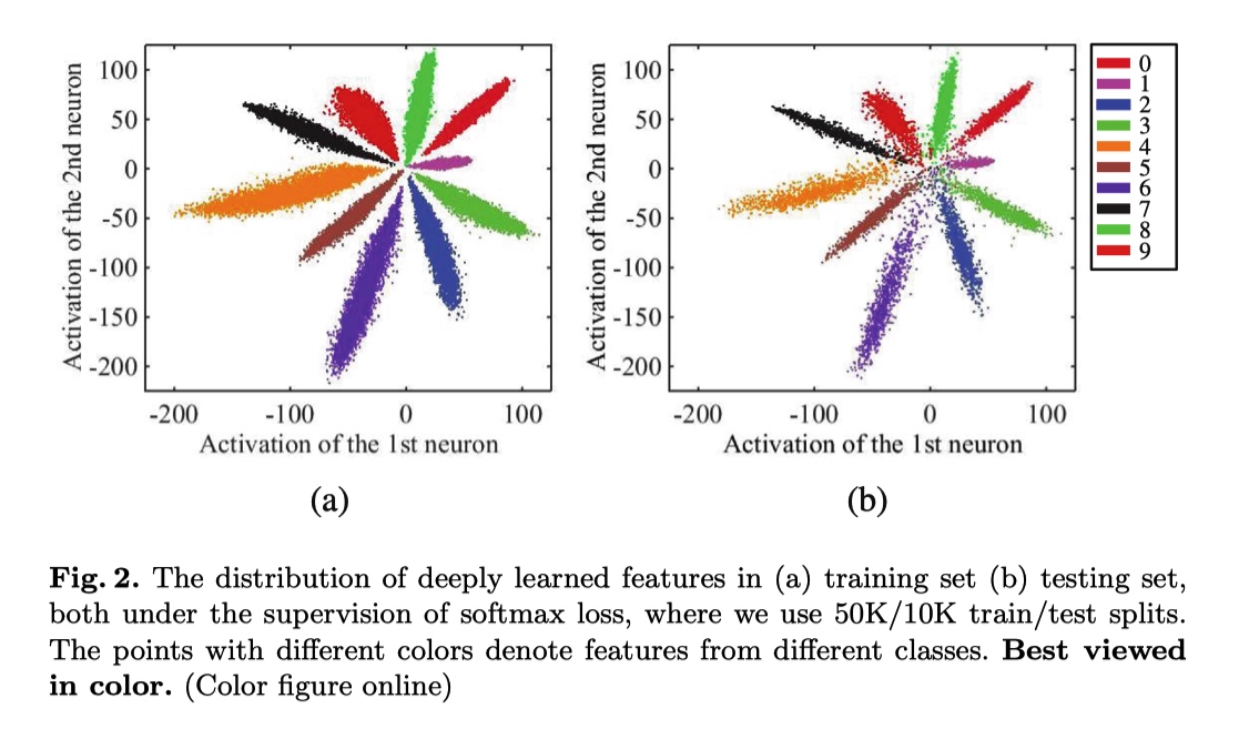
对于人脸识别任务来说，网络学习到的特征具有判别性是一件很重要的事情。增加类间距离，减小类内距离在人脸识别任务中很重要。那么，该如何增加类间距离，减小类内距离呢？通常，我们使用 softmax loss 作为分类任务的 loss, 但是，单单依赖使用 softmax 监督学习到的特征只能将不同类别分开，却无法约束不同类别之间的距离以及类内距离。为了达到增加类间距离，减小类内距离的目的，就需要额外的监督信号，center loss 就是其中一种.

center loss 包含两个流程:

学习一个类别的深度特征的中心
使用该中心约束属于该类别的特征表示

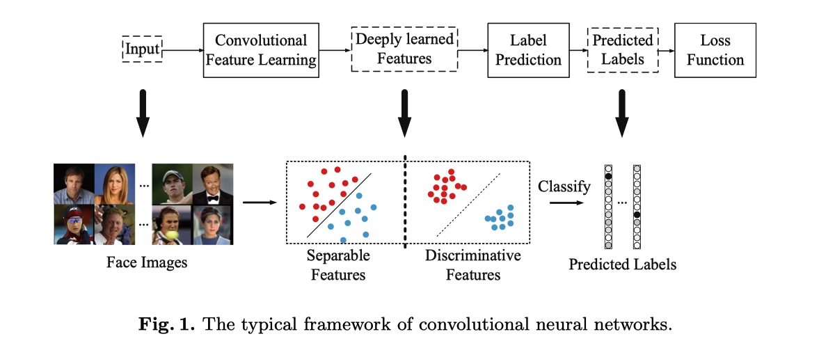
最常用的 CNN 执行特征学习和标签预测，将输入数据映射到深度特征 (最后隐藏层的输出)，然后映射到预测标签，如上图所示。最后一个完全连接层就像一个线性分类器，不同类的深层特征通过决策边界来区分。

center loss design

如何开发一个有效的损失函数来提高深度学习特征的判别力呢？直观地说，最小化类内方差同时保持不同类的特征可分离是关键。

center loss 形式如下:

$c_{y_i} \in R^d$ 为第 $y_i$ 类的特征表示的中心 center 更新策略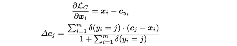

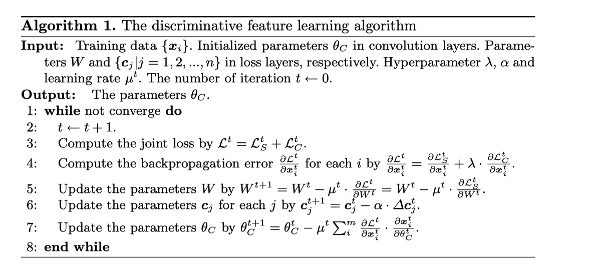
total loss 函数

toy experiment 可视化

超参设置实验

$\lambda \quad$ softmax 与 center loss 的平衡调节因子 $\alpha \quad$ center 学习率，即 $ center -= \alpha \times diff$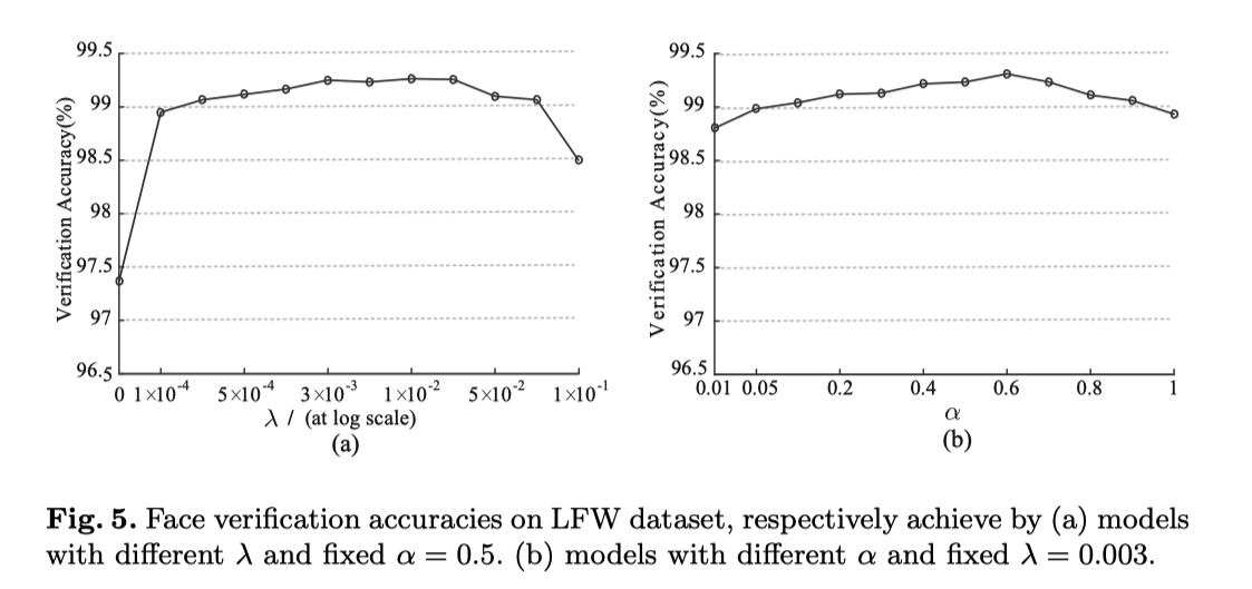

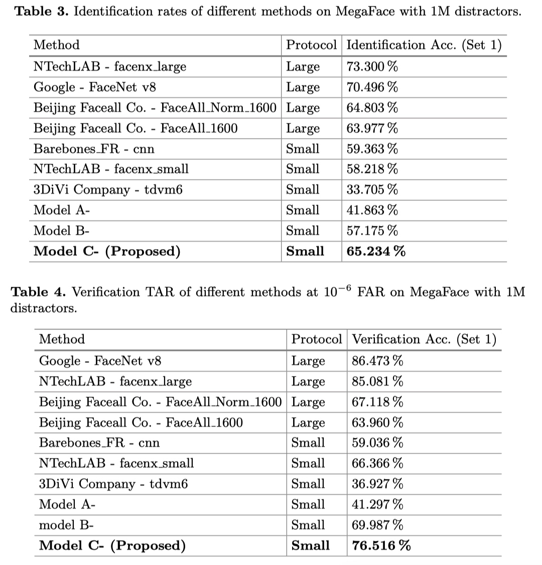
experiment result

thought

就身边的哥们用 center loss 的经验来看，center loss 在用于非人脸识别的任务上，貌似效果一般或者没有效果。可能只有像人脸任务一样，类内深度特征分布聚成一簇的情况下，该 loss 比较有效。如果分类任务中，类内特征差异比较大，可能分为几个小簇 (如年龄预测), 该 loss 可能就没有啥用处了。而且 center loss 没有做特征归一化，不同类的特征表示数量级可能不一样，导致一个数量级比较大特征即使已经很相似了，但是其微小的差距也可能比其他的数量级小的特征的不相似时的的数值大.

而且，学习到的 center 只用于监督训练，在预测过程中不包含任何与 center 的比较过程.

就学习 center 这一思想而言，感觉 cosface 中提到的 large margin cosine loss 中用于学习 feature 与权重之间的 cosine 角度，比较好的实现这种学习一个 center (以 filter 的权重为 center), 然后让 center 尽量与 feature 距离近的思想可能更好一点，即能在训练时规范 feature 与 center 之间的距离，又能在预测时候，通过与 center 比对 cosine 大小来做出预测.

A Gentle Introduction to Transfer Learning for Deep Learning | 迁移学习

by Jason Brownlee on December 20, 2017 in Better Deep Learning

Transfer learning is a machine learning method where a model developed for a task is reused as the starting point for a model on a second task.

It is a popular approach in deep learning where pre-trained models are used as the starting point on computer vision and natural language processing tasks given the vast compute and time resources required to develop neural network models on these problems and from the huge jumps in skill that they provide on related problems.

In this post, you will discover how you can use transfer learning to speed up training and improve the performance of your deep learning model.

After reading this post, you will know:

What transfer learning is and how to use it.
Common examples of transfer learning in deep learning.
When to use transfer learning on your own predictive modeling problems.

Let’s get started.

What is Transfer Learning?

Transfer learning is a machine learning technique where a model trained on one task is re-purposed on a second related task.

Transfer learning and domain adaptation refer to the situation where what has been learned in one setting … is exploited to improve generalization in another setting

— Page 526, Deep Learning, 2016.

Transfer learning is an optimization that allows rapid progress or improved performance when modeling the second task.

Transfer learning is the improvement of learning in a new task through the transfer of knowledge from a related task that has already been learned.

— Chapter 11: Transfer Learning, Handbook of Research on Machine Learning Applications, 2009.

Transfer learning is related to problems such as multi-task learning and concept drift and is not exclusively an area of study for deep learning.

Nevertheless, transfer learning is popular in deep learning given the enormous resources required to train deep learning models or the large and challenging datasets on which deep learning models are trained.

Transfer learning only works in deep learning if the model features learned from the first task are general.

In transfer learning, we first train a base network on a base dataset and task, and then we repurpose the learned features, or transfer them, to a second target network to be trained on a target dataset and task. This process will tend to work if the features are general, meaning suitable to both base and target tasks, instead of specific to the base task.

— How transferable are features in deep neural networks?

This form of transfer learning used in deep learning is called inductive transfer. This is where the scope of possible models (model bias) is narrowed in a beneficial way by using a model fit on a different but related task.

Depiction of Inductive Transfer
Taken from “Transfer Learning”

How to Use Transfer Learning?

You can use transfer learning on your own predictive modeling problems.

Two common approaches are as follows:

Develop Model Approach
Pre-trained Model Approach

Develop Model Approach

Select Source Task. You must select a related predictive modeling problem with an abundance of data where there is some relationship in the input data, output data, and/or concepts learned during the mapping from input to output data.
Develop Source Model. Next, you must develop a skillful model for this first task. The model must be better than a naive model to ensure that some feature learning has been performed.
Reuse Model. The model fit on the source task can then be used as the starting point for a model on the second task of interest. This may involve using all or parts of the model, depending on the modeling technique used.
Tune Model. Optionally, the model may need to be adapted or refined on the input-output pair data available for the task of interest.

Pre-trained Model Approach

Select Source Model. A pre-trained source model is chosen from available models. Many research institutions release models on large and challenging datasets that may be included in the pool of candidate models from which to choose from.
Reuse Model. The model pre-trained model can then be used as the starting point for a model on the second task of interest. This may involve using all or parts of the model, depending on the modeling technique used.
Tune Model. Optionally, the model may need to be adapted or refined on the input-output pair data available for the task of interest.

This second type of transfer learning is common in the field of deep learning.

Examples of Transfer Learning with Deep Learning

Let’s make this concrete with two common examples of transfer learning with deep learning models.

Transfer Learning with Image Data

It is common to perform transfer learning with predictive modeling problems that use image data as input.

This may be a prediction task that takes photographs or video data as input.

For these types of problems, it is common to use a deep learning model pre-trained for a large and challenging image classification task such as the ImageNet 1000-class photograph classification competition.

The research organizations that develop models for this competition and do well often release their final model under a permissive license for reuse. These models can take days or weeks to train on modern hardware.

These models can be downloaded and incorporated directly into new models that expect image data as input.

Three examples of models of this type include:

Oxford VGG Model
Google Inception Model
Microsoft ResNet Model

For more examples, see the Caffe Model Zoo where more pre-trained models are shared.

This approach is effective because the images were trained on a large corpus of photographs and require the model to make predictions on a relatively large number of classes, in turn, requiring that the model efficiently learn to extract features from photographs in order to perform well on the problem.

In their Stanford course on Convolutional Neural Networks for Visual Recognition, the authors caution to carefully choose how much of the pre-trained model to use in your new model.

[Convolutional Neural Networks] features are more generic in early layers and more original-dataset-specific in later layers

— Transfer Learning, CS231n Convolutional Neural Networks for Visual Recognition

Transfer Learning with Language Data

It is common to perform transfer learning with natural language processing problems that use text as input or output.

For these types of problems, a word embedding is used that is a mapping of words to a high-dimensional continuous vector space where different words with a similar meaning have a similar vector representation.

Efficient algorithms exist to learn these distributed word representations and it is common for research organizations to release pre-trained models trained on very large corpa of text documents under a permissive license.

Two examples of models of this type include:

Google’s word2vec Model
Stanford’s GloVe Model

These distributed word representation models can be downloaded and incorporated into deep learning language models in either the interpretation of words as input or the generation of words as output from the model.

In his book on Deep Learning for Natural Language Processing, Yoav Goldberg cautions:

… one can download pre-trained word vectors that were trained on very large quantities of text […] differences in training regimes and underlying corpora have a strong influence on the resulting representations, and that the available pre-trained representations may not be the best choice for [your] particular use case.

— Page 135, Neural Network Methods in Natural Language Processing, 2017.

When to Use Transfer Learning?

Transfer learning is an optimization, a shortcut to saving time or getting better performance.

In general, it is not obvious that there will be a benefit to using transfer learning in the domain until after the model has been developed and evaluated.

Lisa Torrey and Jude Shavlik in their chapter on transfer learning describe three possible benefits to look for when using transfer learning:

Higher start. The initial skill (before refining the model) on the source model is higher than it otherwise would be.
Higher slope. The rate of improvement of skill during training of the source model is steeper than it otherwise would be.
Higher asymptote. The converged skill of the trained model is better than it otherwise would be.

Three ways in which transfer might improve learning.
Taken from “Transfer Learning”.

Ideally, you would see all three benefits from a successful application of transfer learning.

It is an approach to try if you can identify a related task with abundant data and you have the resources to develop a model for that task and reuse it on your own problem, or there is a pre-trained model available that you can use as a starting point for your own model.

On some problems where you may not have very much data, transfer learning can enable you to develop skillful models that you simply could not develop in the absence of transfer learning.

The choice of source data or source model is an open problem and may require domain expertise and/or intuition developed via experience.

Summary

In this post, you discovered how you can use transfer learning to speed up training and improve the performance of your deep learning model.

Specifically, you learned:

What transfer learning is and how it is used in deep learning.
When to use transfer learning.
Examples of transfer learning used on computer vision and natural language processing tasks.

AN EMPIRICAL STUDY OF EXAMPLE FORGETTING DURING DEEP NEURAL NETWORK LEARNING 论文笔记

摘要

　　受到灾难性遗忘现象的启发，我们研究了神经网络在单一分类任务训练时的学习动态。我们的目标是了解当数据没有明显的分布式转变时是否会出现相关现象。我们定义了一个“遗忘事件”
当个别训练示例在学习过程中从正确分类转换为错误时。在几个基准数据集中，我们发现：（i）某些例子被高频率遗忘，有些则完全没有; （ii）数据集的（不）可遗忘的例子概括了神经架构;
（iii）基于遗忘动力学，可以从训练数据集中省略大部分示例，同时仍保持最先进的泛化性能。

简介

　　我们的实验结果表明：a）存在大量令人难忘的例子，即一旦学会就永远不会忘记的例子，这些例子在种子之间是稳定的，并且从一个神经架构到另一个神经架构强烈相关; b）带有嘈杂标签的例子是最被遗忘的例子，还有具有“不常见”特征的图像，视觉上很难分类; c）在数据集上训练神经网络，其中已经移除了大部分最少被遗忘的示例仍然导致测试集上的极具竞争性的性能。

程序描述和实验设置

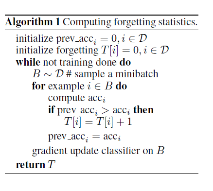
　　根据先前的定义，监视遗忘事件需要在每次模型更新时计算数据集中所有示例的预测，这将非常昂贵。在实践中，对于每个示例，我们通过仅在示例包含在当前小批量中时计算遗忘统计来对完整的遗忘事件序列进行子样本化; 也就是说，我们在随后的小批量中计算遗忘相同示例的演示文稿。这给出了示例在训练期间经历的遗忘事件的数量的下限。

　　我们在给定数据集上训练分类器，并记录每个示例在当前小批量中采样时的遗忘事件。为了进一步分析，我们基于它们经历的遗忘事件的数量对数据集的示例进行排序。从有序数据中采样时，关系会随机中断。从未学过的样本被认为是无数次被遗忘用于分类目的。注意，这种遗忘示例的估计在计算上是昂贵的;

　　我们对三个复杂度日益增加的数据集进行了实验评估：MNIST（LeCun等，1999），置换MNIST - 一种版本的MNIST，其具有应用于所有示例像素的相同固定置换，以及CIFAR10（Krizhevsky，2009）。我们使用各种模型架构和训练方案，产生与各个数据集上当前最新技术水平相当的测试误差。特别是，基于MNIST的实验使用由两个卷积层组成的网络，然后是完全连接的层，使用具有动量和丢失的SGD进行训练。该网络实现0.8％的测试错误。对于CIFAR-10，我们使用带有切口的ResNet（DeVries＆Taylor，2017），使用SGD和动力训练
特定的学习率表。该网络实现了3.99％的竞争性测试错误。

特征样本遗忘

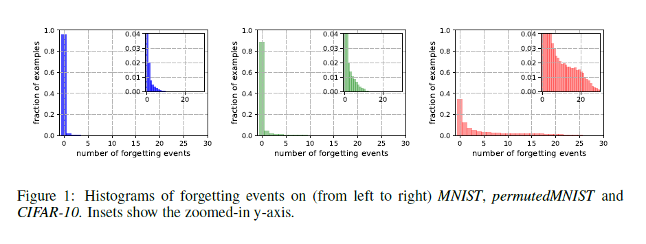
　　遗忘事件的数量。我们估计了5个随机种子中三个不同数据集（MNIST，permuted MNIST和CIFAR-10）的所有训练样例的遗忘事件数。从一个种子计算的遗忘事件的直方图如图1所示。有55012个，45181个和15628个令人难忘的5个种子常见的例子，它们分别代表91.7％，75.3％和31.3％的相应训练集。请注意，具有较少复杂性和多样性的数据集（例如MNIST）似乎包含更多令人难忘的示例。 permuted MNIST表现出MNIST（最简单）和CIFAR-10（最难）之间的复杂性。这一发现似乎暗示了遗忘统计数据与学习问题的内在维度之间的相关性，正如李等人最近提出的那样（2018）。

　　种子间的稳定性。为了测试我们的度量相对于随机梯度下降产生的方差的稳定性，我们计算了10个不同随机种子的每个例子的遗忘事件的数量并测量它们的相关性。从一粒种子到另一粒种子，平均Pearson相关系数为89.2％。当将10个不同的种子随机分成两组5时，这两组中遗忘事件的累积数量显示出97.6％的高相关性。我们还对100个种子进行了原始实验，以设计每个例子中遗忘事件平均数（超过5个种子）的95％置信区间。最少被遗忘的例子的置信区间很紧，确认了具有少量遗忘事件的例子可以自信地提升准确率。

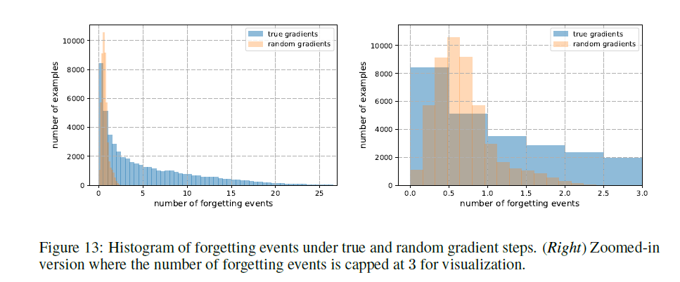
　　偶然遗忘。为了量化偶然发生遗忘的可能性，我们另外分析了在随机更新步骤而不是真正的SGD步骤下获得的遗忘事件的分布。为了保持类似于在SGD期间遇到的随机更新的统计数据，通过在主网络上混合由标准SGD产生的梯度来获得随机更新。我们在补充图13中报告机会遗忘事件的直方图：示例被偶然遗忘了一小部分时间，最多两次，大部分时间不到一次。观察到的种子间的稳定性，机会遗忘事件的数量少以及紧密的置信区间表明，度量产生的排序不太可能是另一个不相关的随机原因的副产品。

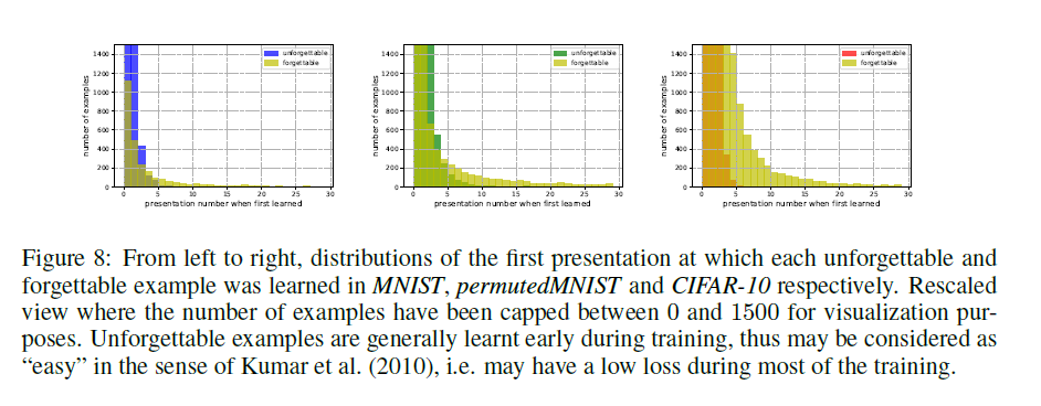
　　第一次学习事件。我们调查是否需要呈现非遗忘和遗忘的例子以便第一次学习（即第一次学习事件发生）。在补充图8中可以看到第一次学习事件在所有数据集中出现的表示编号的分布。我们观察到，虽然难忘和遗忘集都包含许多在前3-4个演示中学习的例子，但是遗忘的例子包含大量先后在训练中学习的示例。第一次学习事件演示与所有训练样例中遗忘事件数量之间的Spearman等级相关性为0.56，表明中等关系。

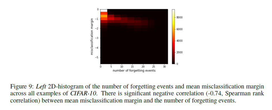
　　错误分类margin。遗忘事件的定义是二元的，因此与更复杂的示例相关性估计量相比较粗略（Zhao＆Zhang，2015; Chang等，2017）。为了确定其有效性，我们计算遗忘事件的误分类边界。一个例子的错误分类界限被定义为所有遗忘事件的平均分类界限，按定义为负数量。示例的遗忘事件数与其平均误分类余量之间的Spearman等级相关性为-0.74（在5个种子上计算，参见补充图9中的相应2D直方图）。这些结果表明，经常被遗忘的例子具有较大的错误分类边际。

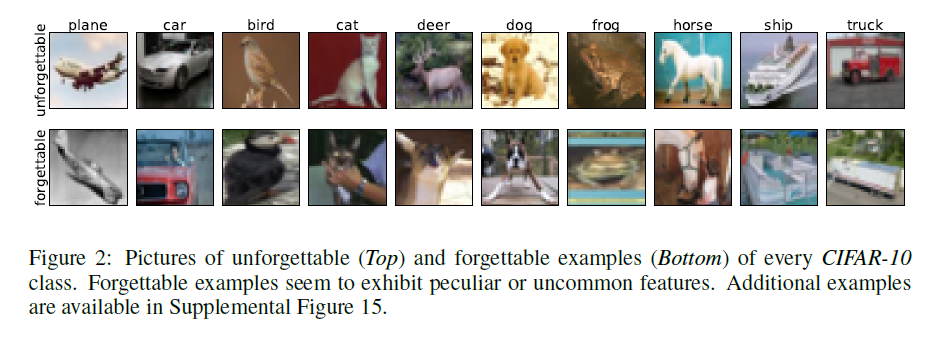
　　视觉检查。我们可视化图2中的一些令人难忘的示例以及CIFAR-10数据集中最遗忘的一些示例。难忘的样本很容易识别并包含最明显的类属性或居中对象，例如晴空中的平面。另一方面，最被遗忘的例子表现出更加模糊的特征（如在中心图像中，棕色背景上的卡车），其可能与来自同一类别的其他示例共有的学习信号不一致。

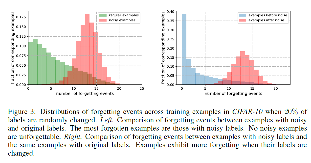
　　检测噪声样本。我们进一步研究了最容易忘记的例子似乎表现出非典型特征的观察结果。我们希望，如果高度遗忘的例子具有非典型的阶级特征，那么噪声样本将会更多地遗忘5个事件。我们随机更改了20％CIFAR-10的标签，并通过训练记录了噪声和常规示例的遗忘事件数。图3显示了在噪声和常规示例中遗忘事件的分布。我们观察到最被遗忘的例子是那些带有噪声标签的例子，没有噪声的例子更难忘。我们还将噪声示例的遗忘事件与具有原始标签的同一组示例的遗忘事件进行比较，并在噪声的情况下观察更高程度的遗忘。这些合成实验的结果支持这样的假设：高度遗忘的例子表现出非典型的类特征。

关于CS224d: Deep Learning for Natural Language Process的介绍已经告一段落，感谢您的耐心阅读，如果想了解更多关于(转) Ensemble Methods for Deep Learning Neural Networks to Reduce Variance and Improve Performance、A Discriminative Feature Learning Approach for Deep Face Recognition、A Gentle Introduction to Transfer Learning for Deep Learning | 迁移学习、AN EMPIRICAL STUDY OF EXAMPLE FORGETTING DURING DEEP NEURAL NETWORK LEARNING 论文笔记的相关信息，请在本站寻找。

本文标签：