本文将带您了解关于Tensorflow--一维离散卷积的新内容，同时我们还将为您解释一维离散卷积怎么算的相关知识，另外，我们还将为您提供关于Centos6安装TensorFlow及TensorFlow

本文将带您了解关于Tensorflow--一维离散卷积的新内容，同时我们还将为您解释一维离散卷积怎么算的相关知识，另外，我们还将为您提供关于Centos6安装TensorFlow及TensorFlowOnSpark、github/tensorflow/tensorflow/contrib/slim/、hello tensorflow，我的第一个tensorflow程序、numpi 与 tensorflow 2.4 上的卷积的实用信息。

• Tensorflow--一维离散卷积（一维离散卷积怎么算）
• Centos6安装TensorFlow及TensorFlowOnSpark
• github/tensorflow/tensorflow/contrib/slim/
• hello tensorflow，我的第一个tensorflow程序
• numpi 与 tensorflow 2.4 上的卷积

Tensorflow--一维离散卷积（一维离散卷积怎么算）

Tensorflow–一维离散卷积

一维离散卷积的运算是一种主要基于向量的计算方式

一.一维离散卷积的计算原理

一维离散卷积通常有三种卷积类型：full卷积，same卷积和valid卷积

1.full卷积

full卷积的计算过程如下：K沿着I顺序移动，每移动一个固定位置，对应位置的值相乘，然后对其求和

其中K称为卷积核或者滤波器或者卷积掩码

2.valid卷积

从full卷积的计算过程可知，如果K靠近I，就会有部分延伸到I之外，valid卷积只考虑能完全覆盖K内的情况，即K在I内部移动的情况

3.same卷积

首先在卷积核K上指定一个锚点，然后将锚点顺序移动到输入张量I的每一个位置处，对应位置相乘然后求和，卷积核锚点的位置一般有以下规则，假设卷积核的长度为FL：

如果FL为奇数，则锚点的位置在(FL-1)/2处

如果FL为偶数，则锚点的位置在(FL-2)/2处

4.full，same，valid卷积的关系

假设一个长度为L的一维张量与一个长度为FL的卷积核卷积，其中Fa代表计算same卷积时，锚点的位置索引，则两者的full卷积与same卷积的关系如下：
Csame=Cfull[FL-Fa-1,FL-Fa+L-2]

full卷积C与valid卷积C的关系如下：
C=C[FL-1,L-1]

same卷积C与valid卷积C的关系如下：
C=C[FL-Fa-2,L-Fa_2]

注意：大部分书籍中对卷积运算的定义分为两步。第1步是将卷积核翻转180；第2步是将翻转的结果沿输入张量顺序移动，每移动到一个固定位置，对应位置相乘然后求和，如Numpy中实现的卷积函数convolve和Scipy中实现的卷积函数convolve，函数内部都进行了以上两步运算。可见，最本质的卷积运算还是在第2步。Tensorflow中实现的卷积函数

tf.nn.conv1d(value,filters,stride,padding,use_cudnn_on_gpu=None,data_format=None,name=None)

其内部就没有进行第1步操作，而是直接进行了第2步操作

import tensorflow as tf

# 输入张量I
I=tf.constant(
    [
        [[3],[4],[1],[5],[6]]  
    ]
    ,tf.float32
)

# 卷积核
K=tf.constant(
    [
        [[-1]],
        [[-2]],
        [[2]],
        [[1]]
    ]
    ,tf.float32
)

I_conv1d_K=tf.nn.conv1d(I,K,1,''SAME'')

session=tf.Session()

print(session.run(I_conv1d_K))

[[[  3.]
  [ -4.]
  [ 10.]
  [  1.]
  [-17.]]]

函数tf.nn.conv1d只实现了same卷积和valid卷积，它就是为更方便地搭建卷积神经网络而设计的。利用Numpy或者Scipy中的卷积函数convolve实现上述示例的full卷积代码如下：

import numpy as np
from scipy import signal

I=np.array([3,4,1,5,6],np.float32)
K=np.array([-1,-2,2,1],np.float32)

# 卷积核K翻转180
K_reverse=np.flip(K,0)
# r=np.convolve(I,K_reverse,mode=''full'')
r=signal.convolve(I,K_reverse,mode=''full'')

print(r)

[  3.  10.   3.  -4.  10.   1. -17.  -6.]

注意：如果卷积核的长度是偶数，函数convolve和tf.nn.conv1d在实现same卷积时，其结果会略有不同，但也只是在边界处(两端)的值有所不同，这是因为这两个函数对卷积核锚点的位置定义不同，本质上就是从full卷积结果中取的区域不一样

二.一维卷积定理

1.一维离散傅里叶变换

Tensorflow通过函数fft和ifft分别实现一维离散的傅里叶变换及逆变换

import tensorflow as tf

# 输入长度为3的一维张量
f=tf.constant([4,5,6],tf.complex64)

session=tf.Session()

# 一维傅里叶变换
F=tf.fft(f)

print("傅里叶变换F的值：")
print(session.run(F))

# 计算F的傅里叶逆变换(显然与输入的f是相等的)
F_ifft=tf.ifft(F)

print("打印F的傅里叶逆变换的值：")
print(session.run(F_ifft))

傅里叶变换F的值：
[15.       -5.9604645e-08j -1.4999998+8.6602545e-01j
 -1.4999999-8.6602563e-01j]
打印F的傅里叶逆变换的值：
[4.+3.9736431e-08j 5.-3.1789145e-07j 6.+0.0000000e+00j]

2.卷积定理

假设有长度为L的一维张量I，I(l)代表I的第l个数，其中0≤l<L，有长度为FL的一维卷积核K，那么I与K的full卷积结果的尺寸为L+FL-1

首先，在I的末尾补零，将I的尺寸扩充到与full卷积尺寸相同，即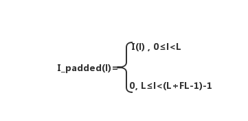

然后，将卷积核K翻转180得到K_rotate180，在末尾进行补零操作，且将K_rotate180的尺寸扩充到和full卷积相同，即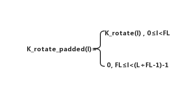

假设fft_Ip和fft_Krp分别是I_padded和K_rotate180_padded的傅里叶变换，那么I☆K的傅里叶变换等于fft_Ipfft_Krp,即

其中代表对应元素相乘，即对应位置的两个复数相乘，该关系通常称为卷积定理

从卷积定理中可以看出分别有对张量的补零操作(或称为边界扩充)和翻转操作。这两种操作在Tensorflow中有对应的函数实现，我们先介绍实现边界扩充的函数：

pad(tensor,padding,mode=''CONSTANT'',name=None,constant_value=0)

以长度为2的一维张量为例，上侧补1个0，下侧补2个0

import tensorflow as tf

x=tf.constant([2,1],tf.float32)

r=tf.pad(x,[[1,2]],mode=''CONSTANT'')

session=tf.Session()

print(session.run(r))

[0. 2. 1. 0. 0.]

当使用常数进行扩充时，也可以选择其他常数，通过参数constant_value进行设置，默认缺省值为0

import tensorflow as tf

x=tf.constant(
    [
        [1,2,3],
        [4,5,6]
    ]
    ,tf.float32
)

# 常数边界扩充，上侧补1行10，下侧补2行10，右侧补1列10
r=tf.pad(x,[[1,2],[0,1]],mode=''CONSTANT'',constant_values=10)

session=tf.Session()

print(session.run(r))

[[10. 10. 10. 10.]
 [ 1.  2.  3. 10.]
 [ 4.  5.  6. 10.]
 [10. 10. 10. 10.]
 [10. 10. 10. 10.]]

除了常数边界扩充，还有其他扩充方式，可以通过参数mode设置，当mode=''SYMMETRIC’时，代表镜像方式的边界扩充；当mode=''REFLECT’时，代表反射方式的边界扩充，可以修改以上程序观察打印结果

Tensorflow通过函数reverse(tensor,axis,name=None)实现张量的翻转，二维张量的每一列翻转(沿"0"方向)，则称为水平镜像；对每一行翻转(沿"1"方向)，则称为垂直镜像

import tensorflow as tf

t=tf.constant(
    [
        [1,2,3],
        [4,5,6]
    ]
    ,tf.float32
)

# 水平镜像
rh=tf.reverse(t,axis=[0])

# 垂直镜像
rv=tf.reverse(t,axis=[1])

# 逆时针翻转180：先水平镜像在垂直镜像(或者先垂直再水平)
r=tf.reverse(t,[0,1])

session=tf.Session()

print("水平镜像的结果：")
print(session.run(rh))
print("垂直镜像的结果：")
print(session.run(rv))
print("逆时针翻转180的结果：")
print(session.run(r))

水平镜像的结果：
[[4. 5. 6.]
 [1. 2. 3.]]
垂直镜像的结果：
[[3. 2. 1.]
 [6. 5. 4.]]
逆时针翻转180的结果：
[[6. 5. 4.]
 [3. 2. 1.]]

掌握了张量边界扩充和翻转的对应函数后，利用卷积定理计算前面中x和K的full卷积

import tensorflow as tf

# 长度为5的输入张量
I=tf.constant(
    [3,4,1,5,6],tf.complex64
)

# 长度为4的卷积核
K=tf.constant(
    [-1,-2,2,1],tf.complex64
)

# 补0操作
I_padded=tf.pad(I,[[0,3]])

# 将卷积核翻转180
K_rotate180=tf.reverse(K,axis=[0])

# 翻转进行0操作
K_rotate180_padded=tf.pad(K_rotate180,[[0,4]])

# 傅里叶变换
I_padded_fft=tf.fft(I_padded)

# 傅里叶变换
K_rotate180_padded_fft=tf.fft(K_rotate180_padded)

# 将以上两个傅里叶变换点乘操作
IK_fft=tf.multiply(I_padded_fft,K_rotate180_padded_fft)

# 傅里叶逆变换
IK=tf.ifft(IK_fft)

# 因为输入的张量和卷积核都是实数，对以上傅里叶逆变换进行取实部的操作
IK_real=tf.real(IK)
session=tf.Session()

print(session.run(IK_real))

[  2.9999998  10.          3.         -4.         10.          1.
 -17.         -6.       ]

三.具备深度的一维离散卷积

1.具备深度的张量与卷积核的卷积

张量x可以理解为是一个长度为3，深度为3的张量，K可以理解为是一个长度为2，深度为3的张量，两者same卷积的过程就是锚点顺序移动到输入张量的每一个位置处，然后对应位置相乘，求和

注意：输入张量的深度和卷积核的深度是相等的

import tensorflow as tf

# 1个长度为3，深度为3的张量
x=tf.constant(
    [
        [[2,5,2],[6,1,-1],[7,9,-5]]
    ]
    ,tf.float32
)

# 1个长度为2，深度为3的卷积核
k=tf.constant(
    [
        [[-1],[5],[4]],[[2],[1],[6]]
    ]
    ,tf.float32
)

# 一维same卷积
v_conv1d_k=tf.nn.conv1d(x,k,1,''SAME'')

session=tf.Session()

print(session.run(v_conv1d_k))

[[[ 38.]
  [-12.]
  [ 18.]]]

2.具备深度的张量分别与多个卷积核的卷积

同一个张量与多个卷积核的卷积本质上是该张量分别与每一个卷积核卷积，然后将每一个卷积结果在深度方向上连接在一起。以长度为3，深度为3的输入张量与2个长度为2，深度为3的卷积核卷积为例

import tensorflow as tf

x=tf.constant(
    [
        [[2,5,2],[6,1,-1],[7,9,-5]]
    ]
    ,tf.float32
)

# 2个长度为2，深度为3的卷积核
k=tf.constant(
    [
        [[-1,1],[5,3],[4,7]],[[2,-2],[1,-1],[6,9]]
    ]
    ,tf.float32
)

v_conv1d_k=tf.nn.conv1d(x,k,1,''SAME'')

session=tf.Session()

print(session.run(v_conv1d_k))

[[[ 38.   9.]
  [-12. -66.]
  [ 18.  -1.]]]

1个深度为C的张量与M个深度为C的卷积核的卷积结果的深度为M，即最后输出结果的深度与卷积核的个数相等

3.多个具备深度的张量分别与多个卷积核的卷积

计算3个长度为3，深度为3的张量与2个长度为2，深度为3的卷积核的卷积

import tensorflow as tf

# 3个长度为3，深度为3的张量
x=tf.constant(
        [
            
            [[2,5,2],[6,1,-1],[7,9,-5]], # 第1个
            [[1,3,2],[5,2,-2],[8,4,3]],  # 第2个
            [[4,5,-1],[1,9,5],[2,7,0]]   # 第3个
        ]
    ,tf.float32
)

# 2个长度为2，深度为3的卷积核
k=tf.constant(
        [
            
            [[-1,1],[5,3],[4,7]],[[2,-2],[1,-1],[6,9]]
        ]
    ,tf.float32
)

v_conv1d_k=tf.nn.conv1d(x,k,1,''SAME'')

session=tf.Session()

print(session.run(v_conv1d_k))

[[[ 38.   9.]
  [-12. -66.]
  [ 18.  -1.]]

 [[ 22.  -6.]
  [ 35.   4.]
  [ 24.  41.]]

 [[ 58.  46.]
  [ 75.  52.]
  [ 33.  23.]]]

函数tf.nn.conv1d可以实现任意多个输入量分别与任意多个卷积核的卷积，输入张量的深度和卷积核的深度是相等的

Centos6安装TensorFlow及TensorFlowOnSpark

1. 需求描述

<property>
                <name>yarn.scheduler.maximum-allocation-mb</name>
                <value>2048</value>
            </property>
        <property>
                <name>yarn.nodemanager.resource.memory-mb</name>
                <value>2048</value>
        </property>
        <property>
                <name>yarn.nodemanager.resource.cpu-vcores</name>
                        <value>2</value>
                            </property>

4. 步骤

安装repo库： yum install -y centos-release-scl
安装 devtoolset:  yum install -y devtoolset-6 

yum install python27 python27-numpy python27-python-devel python27-python-wheel

yum install –y vim zip unzip openssh-clients

先执行：
export CC=/opt/rh/devtoolset-6/root/usr/bin/gcc
接着进入编译环境：
scl enable devtoolset-6 python27 bash
接着以此执行：
 unzip bazel-0.5.1-dist.zip -d bazel-0.5.1-dist
cd bazel-0.5.1-dist

# compile
./compile.sh
 
# install
mkdir -p ~/bin
cp output/bazel ~/bin/

exit  //退出scl环境
// 耗时较久

def tf_extension_linkopts():
  return ["-lrt"]  # No extension link opts

安装基本软件： yum install –y patch
接着，进入编译环境：
scl enable devtoolset-6 python27 bash
cd tensorflow-1.3.0
./configure
 
# build
~/bin/bazel build --config=opt //tensorflow/tools/pip_package:build_pip_package
bazel-bin/tensorflow/tools/pip_package/build_pip_package /tmp/tensorflow_pkg
exit // 退出编译环境
// 耗时同样很久，同样使用bazel0.4.X的版本编译TensorFlow1.3提示版本过低

export PYTHON_ROOT=~/Python // 设置环境变量，并下载Python
curl -O https://www.python.org/ftp/python/2.7.12/Python-2.7.12.tgz
tar -xvf Python-2.7.12.tgz

pushd Python-2.7.12
./configure --prefix="${PYTHON_ROOT}" --enable-unicode=ucs4
make
make install
popd

pushd "${PYTHON_ROOT}"
curl -O https://bootstrap.pypa.io/get-pip.py
bin/python get-pip.py
popd

pushd "${PYTHON_ROOT}"
bin/pip install /tmp/tensorflow_pkg/tensorflow-1.3.0-cp27-none-linux_x86_64.whl
popd

pushd "${PYTHON_ROOT}"
bin/pip install tensorflowonspark
popd

pushd "${PYTHON_ROOT}"
zip -r Python.zip *
popd

hadoop fs -put ${PYTHON_ROOT}/Python.zip

# from __future__ import absolute_import
# from __future__ import division
# from __future__ import print_function

import numpy as np

import tensorflow as tf

X_FEATURE = 'x'  # Name of the input feature.

train_percent = 0.8


def load_data(data_file_name):
    data = np.loadtxt(open(data_file_name),delimiter=",",skiprows=0)
    return data


def data_selection(iris,train_per):
    data,target = np.hsplit(iris[np.random.permutation(iris.shape[0])],np.array([-1]))

    row_split_index = int(data.shape[0] * train_per)

    x_train,x_test = (data[1:row_split_index],data[row_split_index:])
    y_train,y_test = (target[1:row_split_index],target[row_split_index:])
    return x_train,x_test,y_train.astype(int),y_test.astype(int)


def run():
    # Load dataset.
    data_file = 'iris01.csv'
    iris = load_data(data_file)
    # x_train,y_train,y_test = model_selection.train_test_split(
    #     iris.data,iris.target,test_size=0.2,random_state=42)

    x_train,y_test = data_selection(iris,train_percent)

    # print(x_test)
    # print(y_test)

    #
    # # Build 3 layer DNN with 10,20,10 units respectively.
    feature_columns = [
        tf.feature_column.numeric_column(
            X_FEATURE,shape=np.array(x_train).shape[1:])]
    classifier = tf.estimator.DNNClassifier(
        feature_columns=feature_columns,hidden_units=[10,10],n_classes=3)
    #
    # # Train.
    train_input_fn = tf.estimator.inputs.numpy_input_fn(
        x={X_FEATURE: x_train},y=y_train,num_epochs=None,shuffle=True)
    classifier.train(input_fn=train_input_fn,steps=200)
    #
    # # Predict.
    test_input_fn = tf.estimator.inputs.numpy_input_fn(
        x={X_FEATURE: x_test},y=y_test,num_epochs=1,shuffle=False)
    predictions = classifier.predict(input_fn=test_input_fn)
    y_predicted = np.array(list(p['class_ids'] for p in predictions))
    y_predicted = y_predicted.reshape(np.array(y_test).shape)
    # #
    # # # score with sklearn.
    # score = metrics.accuracy_score(y_test,y_predicted)
    # print('Accuracy (sklearn): {0:f}'.format(score))
    print(np.concatenate(( y_predicted,y_test),axis= 1))
    # score with tensorflow.
    scores = classifier.evaluate(input_fn=test_input_fn)
    print('Accuracy (tensorflow): {0:f}'.format(scores['accuracy']))

    print(classifier.params)


if __name__ == '__main__':
    run()

5.1,3.5,1.4,0.2,0
4.9,3.0,0
4.7,3.2,1.3,0
4.6,3.1,1.5,0
5.0,3.6,0
5.4,3.9,1.7,0.4,3.4,0.3,0
4.4,2.9,0.1,3.7,0
4.8,1.6,0
4.3,1.1,0
5.8,4.0,1.2,0
5.7,4.4,0
5.1,3.8,1.0,3.3,0.5,1.9,0
5.2,4.1,0
5.5,4.2,0
4.5,2.3,0.6,0
5.3,0
7.0,4.7,1
6.4,4.5,1
6.9,4.9,1
5.5,1
6.5,2.8,4.6,1
5.7,1
6.3,1
4.9,2.4,1
6.6,1
5.2,2.7,1
5.0,2.0,1
5.9,1
6.0,2.2,1
6.1,1
5.6,1
6.7,1
5.8,1
6.2,2.5,4.8,1.8,4.3,1
6.8,5.0,2.6,5.1,1
5.4,1
5.1,6.0,2
5.8,2
7.1,5.9,2.1,2
6.3,5.6,2
6.5,5.8,2
7.6,6.6,2
4.9,2
7.3,6.3,2
6.7,2
7.2,6.1,2
6.4,5.3,2
6.8,5.5,2
5.7,2
7.7,6.7,6.9,2
6.0,2
6.9,5.7,2
5.6,2
6.2,2
6.1,2
7.4,2
7.9,6.4,5.4,5.2,2
5.9,2

from pyspark.context import SparkContext
from pyspark.conf import SparkConf
from tensorflowonspark import TFCluster,TFNode
#from com.yahoo.ml.tf import TFCluster,TFNode
from datetime import datetime

sc = SparkContext(conf=SparkConf().setAppName("your_app_name"))
    num_executors = int(sc._conf.get("spark.executor.instances"))
    num_ps = 1
    tensorboard = True

    cluster = TFCluster.run(sc,run,sys.argv,num_executors,num_ps,tensorboard,TFCluster.InputMode.TENSORFLOW)
    cluster.shutdown()

# from __future__ import absolute_import
# from __future__ import division
# from __future__ import print_function
from pyspark.context import SparkContext
from pyspark.conf import SparkConf
from tensorflowonspark import TFCluster,TFNode
from datetime import datetime
import numpy as np
import sys
# from sklearn import metrics
# from sklearn import model_selection

import tensorflow as tf

X_FEATURE = 'x'  # Name of the input feature.

train_percent = 0.8


def load_data(data_file_name):
    data = np.loadtxt(open(data_file_name),y_test.astype(int)


def map_run(argv,ctx):
    # Load dataset.
    data_file = 'iris01.csv'
    iris = load_data(data_file)
    # x_train,axis= 1))
    # score with tensorflow.
    scores = classifier.evaluate(input_fn=test_input_fn)
    print('Accuracy (tensorflow): {0:f}'.format(scores['accuracy']))

    print(classifier.params)


if __name__ == '__main__':
    import tensorflow as tf
    import sys
    sc = SparkContext(conf=SparkConf().setAppName("your_app_name"))
    num_executors = int(sc._conf.get("spark.executor.instances"))
    num_ps = 1
    tensorboard = False

    cluster = TFCluster.run(sc,map_run,TFCluster.InputMode.TENSORFLOW)
    cluster.shutdown()	

export PYTHON_ROOT=./Python
export LD_LIBRARY_PATH=${PATH}
export PYSPARK_PYTHON=${PYTHON_ROOT}/bin/python
export SPARK_YARN_USER_ENV="PYSPARK_PYTHON=Python/bin/python"
export PATH=${PYTHON_ROOT}/bin/:$PATH
#export QUEUE=gpu

# set paths to libjvm.so,libhdfs.so,and libcuda*.so
#export LIB_HDFS=/opt/cloudera/parcels/CDH/lib64                      # for CDH (per @wangyum)
export LIB_HDFS=$HADOOP_PREFIX/lib/native
export LIB_JVM=$JAVA_HOME/jre/lib/amd64/server
#export LIB_CUDA=/usr/local/cuda-7.5/lib64

# for cpu mode:
 export QUEUE=default

/usr/local/spark-1.5.1-bin-hadoop2.6/bin/spark-submit --master yarn --deploy-mode cluster --num-executors 3 --executor-memory 1024m --archives hdfs://s0:8020/user/root/Python.zip#Python,/root/iris01.csv /root/iris_c.py

5. 问题及解决

6. 总结

github/tensorflow/tensorflow/contrib/slim/

TensorFlow-Slim

TF-Slim 是一个轻量级的库，用来在 TF 中定义、训练和评估复杂模型。tf-slim 能够自由混入原生 TF 和其它框架（如 tf.contrib.learn 中）。

用法

import tensorflow.contrib.slim as slim

为什么用 TF-Slim?

TF-Slim 中都有什么组成部分？

定义模型

变量

层

Scopes

实例：实现 VGG16

训练模型

Training Tensorflow models requires a model, a loss function, the gradient computation and a training routine that iteratively computes the gradients of the model weights relative to the loss and updates the weights accordingly. TF-Slim provides both common loss functions and a set of helper functions that run the training and evaluation routines.

损失

The loss function defines a quantity that we want to minimize. For classification problems, this is typically the cross entropy between the true distribution and the predicted probability distribution across classes. For regression problems, this is often the sum-of-squares differences between the predicted and true values.

Certain models, such as multi-task learning models, require the use of multiple loss functions simultaneously. In other words, the loss function ultimately being minimized is the sum of various other loss functions. For example, consider a model that predicts both the type of scene in an image as well as the depth from the camera of each pixel. This model''s loss function would be the sum of the classification loss and depth prediction loss.

TF-Slim provides an easy-to-use mechanism for defining and keeping track of loss functions via the losses module. Consider the simple case where we want to train the VGG network:

Training Loop

TF-Slim provides a simple but powerful set of tools for training models found in learning.py. These include a Train function that repeatedly measures the loss, computes gradients and saves the model to disk, as well as several convenience functions for manipulating gradients. For example, once we''ve specified the model, the loss function and the optimization scheme, we can call slim.learning.create_train_op and slim.learning.train to perform the optimization:

实例：训练 VGG16 模型

To illustrate this, let''s examine the following sample of training the VGG network:

微调已存在的模型

Brief Recap on Restoring Variables from a Checkpoint

After a model has been trained, it can be restored using tf.train.Saver() which restores Variables from a given checkpoint. For many cases, tf.train.Saver() provides a simple mechanism to restore all or just a few variables.

Partially Restoring Models

It is often desirable to fine-tune a pre-trained model on an entirely new dataset or even a new task. In these situations, one can use TF-Slim''s helper functions to select a subset of variables to restore:

Restoring models with different variable names

Fine-Tuning a Model on a different task

Consider the case where we have a pre-trained VGG16 model. The model was trained on the ImageNet dataset, which has 1000 classes. However, we would like to apply it to the Pascal VOC dataset which has only 20 classes. To do so, we can initialize our new model using the values of the pre-trained model excluding the final layer:

评估模型

Once we''ve trained a model (or even while the model is busy training) we''d like to see how well the model performs in practice. This is accomplished by picking a set of evaluation metrics, which will grade the model''s performance, and the evaluation code which actually loads the data, performs inference, compares the results to the ground truth and records the evaluation scores. This step may be performed once or repeated periodically.

度量

我们定义一个度量来衡量训练效果，这不是一个损失函数（损失被用来在训练过程中进行优化的）。例如，我们训练时最小化 log 损失，但是评估模型时我们也许会用 F1 score , 或者 Intersection Over Union score（这个值不可微，因此也不能用在损失函数上）。

TF-Slim 提供了一组度量 operations。笼统地讲，计算一个度量值可以被分为三部分：

1. 初始化：初始化用来计算度量的变量。
2. Aggregation: perform operations (sums, etc) used to compute the metrics.
3. Finalization: (optionally) perform any final operation to compute metric values. For example, computing means, mins, maxes, etc.

例如，计算 mean_absolute_error，两个变量 (count 和 total) 被初始化为 0。在 aggregation，我们得到一组 predictions 和 labels，计算它们的绝对误差并总计为 total。我们每增加一组，count也随之增加。最后，在 finalization 阶段 ，total 除以 count 来获得均值。

The following example demonstrates the API for declaring metrics. Because metrics are often evaluated on a test set which is different from the training set (upon which the loss is computed), we''ll assume we''re using test data:

images, labels = LoadTestData(...)
predictions = MyModel(images)

mae_value_op, mae_update_op = slim.metrics.streaming_mean_absolute_error(predictions, labels)
mre_value_op, mre_update_op = slim.metrics.streaming_mean_relative_error(predictions, labels)
pl_value_op, pl_update_op = slim.metrics.percentage_less(mean_relative_errors, 0.3)

就像例子描述的那样，创建的 metric 返回两个值： value_op 和 update_op。 value_op 是一个 idempotent operation 返回 metric 的当前值。update_op 是一个 operation，它执行 aggregation 步骤 并返回 metric 的值。

跟踪 value_op 和 update_op 费时费力。为了解决这个问题，TF-Slim 提供两个方便的函数：

# 总计value和update ops 到两个列表中:
value_ops, update_ops = slim.metrics.aggregate_metrics(
    slim.metrics.streaming_mean_absolute_error(predictions, labels),
    slim.metrics.streaming_mean_squared_error(predictions, labels))

# 总起value和update ops 到两个字典中:
names_to_values, names_to_updates = slim.metrics.aggregate_metric_map({
    "eval/mean_absolute_error": slim.metrics.streaming_mean_absolute_error(predictions, labels),
    "eval/mean_squared_error": slim.metrics.streaming_mean_squared_error(predictions, labels),
})

hello tensorflow，我的第一个tensorflow程序

上代码：

import tensorflow as tf

if __name__==''__main__'': 
    g = tf.Graph()   
    # add ops to the user created graph
    with g.as_default(): 
        hello = tf.constant(''Hello Tensorflow'') 
        sess = tf.compat.v1.Session(graph=g)
        print(sess.run(hello)) 

输出如下图右侧：

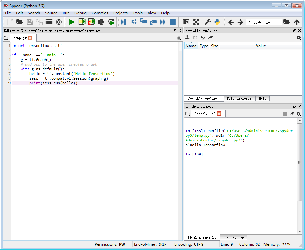
说明：python3.7.4 ，tensorflow2.0 

 若对您有用，请赞助个棒棒糖~

numpi 与 tensorflow 2.4 上的卷积

虽然我认为这个问题大部分是 this question 的重复，但我可以用这个问题来想出一个等效的脚本。

import tensorflow as tf
import numpy as np

I = [3,4,5]
K = [2,1,0]

I = [0] + I + [0]

i = tf.constant(I,dtype=tf.float32,name='i')
k = tf.constant(K,name='k')

data   = tf.reshape(i,[1,int(i.shape[0]),1],name='data')
kernel = tf.reshape(k,[int(k.shape[0]),name='kernel')

res = tf.squeeze(tf.nn.conv1d(data,kernel[::-1],'SAME'))
print(res)
print(np.convolve(I,K,'SAME'))

tf.Tensor([ 6. 11. 14. 5. 0.],shape=(5,),dtype=float32)

[ 6 11 14 5 0]

在您的情况下，他们的关键是了解 tensorflow 和 numpy 如何处理填充。尽管链接的问题很好地解释了这一点，但我还要注意到一个事实，即 full 的默认 np.convolve 填充在 tensorflow conv 1d 中没有等效项。

关于Tensorflow--一维离散卷积和一维离散卷积怎么算的问题我们已经讲解完毕，感谢您的阅读，如果还想了解更多关于Centos6安装TensorFlow及TensorFlowOnSpark、github/tensorflow/tensorflow/contrib/slim/、hello tensorflow，我的第一个tensorflow程序、numpi 与 tensorflow 2.4 上的卷积等相关内容，可以在本站寻找。